Convolutional Neural Networks

[math] \newcommand{\ul}{\mathbf} \newcommand{\symbf}{\bm} \newcommand\subsetap{\mathrel{\overset{\makebox[0pt]{\mbox{\normalfont\tiny\sffamily ap.}}}{\rule{0pt}{.8ex}\smash{\subset}}}} \newcommand{\rident}[1]{\mathrm{#1}} \newcommand{\iident}[1]{\mathit{#1}} \newcommand{\wip}{\emoji{construction}} \newcommand{\pointright}{\emoji{backhand-index-pointing-right-light-skin-tone}} \DeclareMathOperator*{\argmax}{arg\,max} \DeclareMathOperator*{\argmin}{arg\,min} \DeclareMathOperator*{\Arg}{Arg} \DeclareMathOperator*{\Var}{Var} \DeclareMathOperator*{\dom}{dom} \DeclareMathOperator{\Div}{div} \DeclareMathOperator{\morph}{\scalebox{0.7}{\ensuremath\square}} \DeclareMathOperator*{\esssup}{ess\,sup} \DeclareMathOperator{\Int}{Int} \DeclareMathOperator{\Cl}{Cl} \DeclareMathOperator{\id}{id} \DeclareMathOperator{\diam}{diam} \DeclareMathOperator{\supp}{supp} \DeclareMathOperator{\arctantwo}{arctan2} \DeclareMathOperator{\relu}{ReLU} \newcommand{\mathds}{\mathbb}[/math]

This article was automatically generated from a tex file and may contain conversion errors. If permitted, you may login and edit this article to improve the conversion.

[math]\rightarrow[/math] Visualizations of convolutions from , also available at [1].

[math]\rightarrow [/math] Handy reference that provides an overview of CNNs: CNN cheat-sheet.

We previously saw that using fully connected networks for high dimensional data such as images is a non-starter due to the memory and computational requirements involved. The proposed solution was reducing the effective amount of parameters by a combination of using a sparse matrix and weight sharing/parameterization. How exactly we should sparsify the network and which weights should be shared or parametrized had to be determined application by application. In this section we will look at a combination of sparsity and weight sharing that is suited to data that has a natural spatial structure, think about signals in time (1D), images (2D) or volumetric data (3D). What these types of spatial data have in common is that we treat each `part' of the input data in the same way, e.g. we do not process the left side of an image in another way than the right side. The type of network that exploits this spacial structure is called a Convolutional Neural Networks, or CNN for short. As the name suggest these networks employ the convolution operation as well as the closely related pooling operation. We will look at how discrete convolution and pooling are defined and how they are used to construct a deep CNN.

Discrete Convolution

Recall that in the familiar continuous setting the convolution of two functions [math]f,g : \mathbb{R} \to \mathbb{R}[/math] is defined as:

[[math]] \begin{equation} \label{eq:classic_convolution} (f * g)(x) := \int_{\mathbb{R}} f(x-y) \, g(y) \, d y , \end{equation} [[/math]]

which can be interpreted as a filter (or kernel) [math]f[/math] being translated over the data [math]g[/math] and at each translated location the [math]L^2[/math] inner product is taken. To switch to the discrete setting we will use notation that is more in line with programming languages. When we have [math]f \in \mathbb{R}^n[/math] we will use square brackets and zero-based indexing to access its components, so [math]f[0] \in \mathbb{R}[/math] is [math]f[/math]'s first component and [math]f[n-1] \in \mathbb{R}[/math] its last. We use this array-based notation since we will need to do some computations on indices and [math]f[i-j+1][/math] is easier to read than [math]f_{i-j+1}[/math]. Example

Let [math]x \in \mathbb{R}^n[/math], [math]y \in \mathbb{R}^m[/math] and [math]A \in \mathbb{R}^{m \times n}[/math] then the familiar matrix product [math]y=Ax[/math] can be written in array notation as

[[math]] \begin{equation*} y[i] = \sum_{j=0}^{n-1} A[i,j] \, x[j] \end{equation*} [[/math]]

for each [math]i \in \{ 0,\ldots,m-1 \}[/math].

Definition (Discrete cross-correlation and convolution in 1D)

Let [math]f \in \mathbb{R}^n[/math] (the input) and [math]k \in \mathbb{R}^m[/math] (the kernel) then their discrete cross-correlation [math](k \star f) \in \mathbb{R}^{n-m+1}[/math] is given by:

[[math]] \begin{equation*} (k \star f)[i] := \sum_{j=0}^{m-1} k[j] \, f[i+j] \end{equation*} [[/math]]

for [math]i \in \{ 0, \ldots, n-m \}[/math]. Discrete convolution is defined similarly but with one of the inputs reversed:

[[math]] \begin{equation*} (k * f)[i] := \sum_{j=0}^{m-1} k[m-1-j] \, f[i+j] \end{equation*} [[/math]]

for [math]i \in \{ 0, \ldots, n-m \}[/math].

Making an index substitution in the definition of discrete convolution makes the relation to the continuous convolution \ref{eq:classic_convolution} more apparent:

[[math]] \begin{equation*} (k * f)[i] = \sum_{j=i}^{i+m-1} k[i-j + (m-1)] \, f[j] . \end{equation*} [[/math]]

The idea here is to let the components of the kernel [math]k \in \mathbb{R}^m[/math] be trainable parameters. In that context it does not matter whether the kernel is reflected or not and there is no real reason to distinguish convolution from cross-correlation. Consequently in the deep learning field it is usual to refer to both operations as convolution. Most `convolution' operators in deep learning software are in fact implemented as cross-correlations, as in PyTorch for example. We will adopt the same convention and talk about such subjects as convolution layers and convolutional neural networks but the actual underlying operation we will use is cross-correlation. As in the continuous case, discrete convolution can be generalized to higher dimensions. For this course we will only look at the 2 dimensional case as extending to higher dimensions is straightforward. To make things slightly simpler we will restrict ourselves to square kernels, in practice kernels are almost always chosen to be square anyway.

Definition

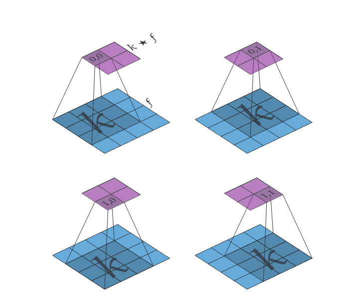
(Discrete cross-correlation in 2D) Let [math]f \in \mathbb{R}^{h \times w}[/math] (the input, read [math]h[/math] as height and [math]w[/math] as width) and [math]k \in \mathbb{R}^{m \times m}[/math] (the kernel) then their discrete cross-correlation [math](k \star f) \in \mathbb{R}^{(h-m+1) \times (w-m+1)}[/math] is given by

[[math]] \begin{equation*} (k \star f)[i_1, i_2] := \sum_{j_1,j_2=0}^{m-1} k[j_1,j_2] \, f[i_1 + j_1, i_2 + j_2] \end{equation*} [[/math]]

for [math]i_1 \in \{ 0,\ldots, h-m \}[/math] and [math]i_2 \in \{ 0, \ldots, w-m \}[/math].

The convolution operator “*” can be extended to 2 dimensions similarly but we will only be using cross-correlation for the remainder of our discussion of convolutional neural networks. For a visualization of discrete convolution in 2D, see Figure figure.

An illustration of convolution (or cross-correlation) in 2D. Here the input [math]f \in \mathbb{R}^{4 \times 4}[/math] (colored blue) is convolved with the kernel [math]k \in \mathbb{R}^{3 \times 3}[/math], which yields an output [math](k \star f) \in \mathbb{R}^{2 \times 2}[/math] (colored purple).

Remark [Index interpretation conventions]

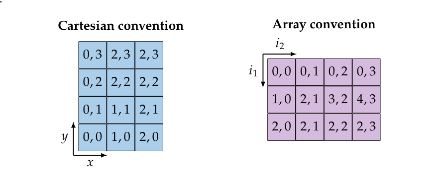
In Definition we called the first dimension of an array [math]f \in \mathbb{R}^{h \times w}[/math] the height and the second the width. Additionally, if you look at Figure we place the origin point [math](0,0)[/math] in the top left. This is different to the Cartesian convention of denoting points in the plane with [math](x,y)[/math] (i.e. width first, height second) and having the origin in the bottom left. Both conventions are illustrated bellow for an element of [math]\mathbb{R}^{3 \times 4}[/math].

Of course choosing either convention does not change the underlying object, merely the interpretation of the indices and shape in colloquial terms. The array convention is almost universally adopted in software and it is used in PyTorch, for that reason we will adopt it when dealing with spatial data.

Padding

The convolution operations we proposed so far have the property that the output is of smaller size than the input. Depending on our goal this might or might not be desirable. If shrinking output size is not desirable we can use padding to ensure the output size is the same as the input size. The most common type of padding is zero padding, which we will look at for the 2 dimensional case.

Definition (Zero padding in 2D)

Let [math]f \in \mathbb{R}^{h \times w}[/math] and let [math]p_t,p_b,p_l,p_r[/math], which we read as top, bottom, left and right padding respectively. Then we define [math]\iident{ZP}_{p_t,p_b,p_l,p_r} f \in \mathbb{R}^{(h+p_t+p_b)\times(w+p_l+p_r)}[/math] as

[[math]] \begin{equation*} \iident{ZP}_{p_t,p_b,p_l,p_r} f [i_1,i_2] := \begin{cases} 0 \qquad & \text{if } i_1 \lt p_t \text{ or } i_1 \geq h + p_t \\ & \text{ or } i_2 \lt p_l \text{ or } i_2 \geq w + p_l, \\ f[i_1-p_t,\,i_2-p_l] & \text{else,} \end{cases} \end{equation*} [[/math]]

for all [math]i_1 \in \{ 0,\ldots,h+p_t+p_b-1 \}[/math] and [math]i_2 \in \{0,\ldots,w+p_l+p_r-1 \}[/math].

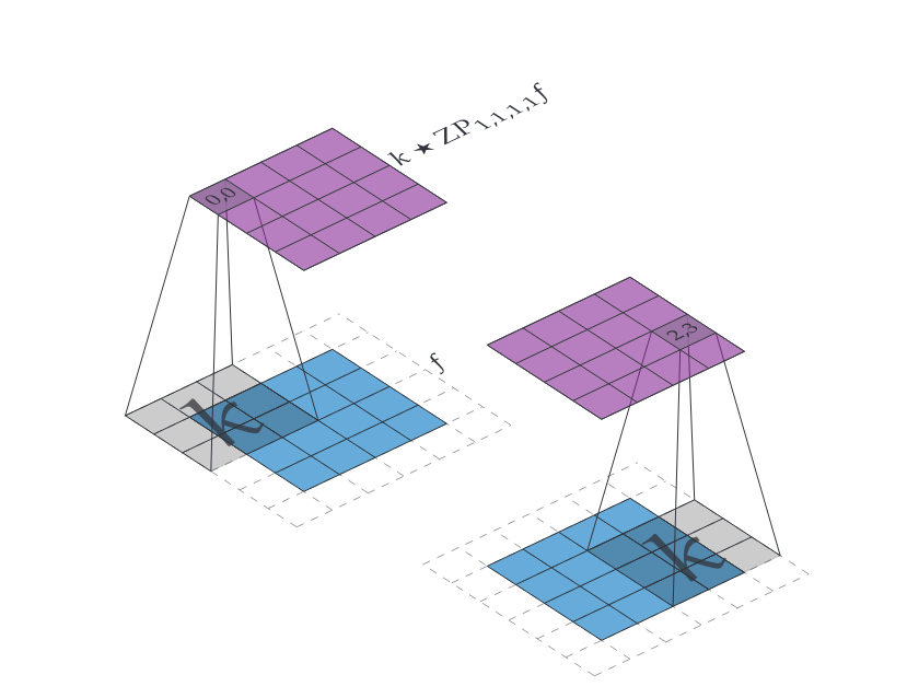
If we then have an [math]f \in \mathbb{R}^{h \times w}[/math] and we want to convolve with a kernel [math]\mathbb{R}^{m \times m}[/math] while keeping the shape of the output the same we can choose

[[math]] \begin{equation*} p_t := \left\lfloor \frac{m-1}{2} \right\rfloor ,\quad p_b := \left\lceil \frac{m-1}{2} \right\rceil ,\quad p_l := \left\lfloor \frac{m-1}{2} \right\rfloor ,\quad p_r := \left\lceil \frac{m-1}{2} \right\rceil , \end{equation*} [[/math]]

then [math]k \star \iident{ZP}_{p_t,p_b,p_l,p_r} f \in \mathbb{R}^{h \times w}[/math]. We leave verifying this claim as an exercise. An example of this technique is illustrated in Figure figure.

Adding padding to the input allows the output of the convolution operation to retain the size of the original input. The most common type of padding is zero-padding, where each out-of-bounds value is assumed to be zero.

Many more padding techniques exist, they only vary in how the out-of-bounds values are chosen. In PyTorch the available padding modes are listed in pytorch.org/docs/stable/generated/torch.nn.functional.pad.html.

Max Pooling

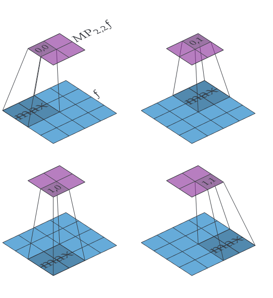
The second operation commonly found in CNN is max pooling. We already saw an activation function called max pooling previously, this is exactly what is used in a CNN but with a particular choice of subsets to take maxima over that plays well with the spatial structure of the data. The idea is to have a `window' slide over the input data in the same way that a convolution kernel slides over the data and then take the maximum value in each window. We will take a look at a particular type of 2D max pooling that is commonly found in CNNs used for image processing and classification applications.

Definition ([math]m \times m[/math] max pooling in 2D)

Let [math]f \in \mathbb{R}^{h \times w}[/math] and let [math]m \in \mathbb{N}[/math]. Then we define [math]\iident{MP}_{m,m} f \in \mathbb{R}^{\lfloor\frac{h}{m}\rfloor \times \lfloor\frac{w}{m}\rfloor}[/math] as

[[math]] \begin{equation*} \iident{MP}_{m,m} f [i_1,i_2] := \max_{\substack{ 0 \leq j_1 \lt m \\ 0 \leq j_2 \lt m }} f[ i_1 m + j_1, i_2 m + j_2] \end{equation*} [[/math]]

for all [math]i_1 \in \{ 0 ,\ldots, \lfloor\frac{h}{m}\rfloor \}[/math] and [math]i_2 \in \{ 0 ,\ldots, \lfloor\frac{w}{m}\rfloor \}[/math].

Two things to note about this particular definition. First, if [math]h[/math] and/or [math]w[/math] is not divisible by [math]m[/math] then some values at the edges will be ignored entirely and not contribute to the output. We could modify the definition to resolve this but in practice [math]m[/math] is usually set to [math]2[/math] and so in the worst case we lose a single row of values at the edge, and that is only if the input has odd dimensions. Second, we move the window in steps of [math]m[/math] in both directions instead of taking steps of [math]1[/math], this is called having a stride of [math]m[/math]. Having a stride larger than [math]1[/math] allows max pooling to quickly reduce the dimensions of the data. Figure figure shows an example of how [math]\iident{MP}_{2,2}[/math] works.

Max pooling is similar to convolution in that a window of a certain size slides over the input, instead of taking a weighted sum inside the window we take the maximum value. Usually the window is moved in strides equal to its size so that the outputs are the maxima from disjoint sets of the input. The pooling operation in the figure is usually just called [math]2 \times 2[/math] max pooling, referring to both the window size and stride used.

Convolutional Layers

So how are convolutions/cross-correlations used in a neural network? First of all we organize our inputs and outputs differently, instead of the inputs and outputs being element of [math]\mathbb{R}^n[/math] for some [math]n[/math] we want to keep the spatial structure. In the 2D case it makes sense to talk about objects with height and width, so elements in [math]\mathbb{R}^{h \times w}[/math] for some choice of [math]h,w \in \mathbb{N}[/math]. We will call these objects 2D maps or just maps. We will want more than one map at any stage of the network, we say we want multiple channels. Concretely, say we have a deep network where we index the number of layers with [math]i[/math], then we denote the input of layer [math]i[/math] as an element in [math]\mathbb{R}^{C_{i-1} \times h_{i-1} \times w_{i-1}}[/math] and the output of layer [math]i[/math] as an element of [math]\mathbb{R}^{C_{i} \times h_{i} \times w_{i}}[/math]. We say layer [math]i[/math] has [math]C_{i-1}[/math] input channels and [math]C_{i}[/math] output channels. We call [math]h_{i-1}\times w_{i-1}[/math] and [math]h_i \times w_i[/math] the shape of the input respectively output maps.

Example [Image inputs] If we design a neural network to process color 1080p images then [math]C_0=3[/math] (RGB images have 3 color channels), [math]h_0=1080[/math] and [math]w_0=1920[/math], i.e. the input to the first layer is an element in [math]\mathbb{R}^{3 \times 1080 \times 1920}[/math]. For a monochrome image we would need just 1 channel.

A convolution layer is just a specialized network layer, hence it follows the same pattern of first doing a linear transform, then adding a bias and finally applying an activation function. The activation function in a CNN is typically a ReLU or max pooling function (or both). The linear part will consist of taking convolutions of the input maps, but there are several ways to do that, we will look at two of them. The first, and most straightforward one, is called single channel convolution (alternatively know as depthwise convolution). With this method we assign a kernel of a certain size to each input channel and then perform the convolution of each input channel with each kernel. This gives us a number of maps equal to the number of input channels, we subsequently take point-wise linear combinations of those maps to generate the desired number of output maps.

Definition (Single channel convolution)

Let [math]f \in \mathbb{R}^{C \times h \times w}[/math] and let [math]k \in \mathbb{R}^{C \times m \times m}[/math]. We call [math]C[/math] the number of input channels, [math]h \times w[/math] the input map shape and [math]m \times m[/math] the kernel shape. Let [math]A \in \mathbb{R}^{C' \times C}[/math], we call [math]C'[/math] the number of output channels. Then we define [math]SCC_{k,A}(f) \in \mathbb{R}^{C' \times (h-m+1) \times (w-m+1)}[/math] as:

[[math]] \begin{equation*} \iident{SCC}_{k,A}(f)[c',i_1,i_2] := \sum_{c=0}^{C-1} A[c',c] \ k[c,\cdot,\cdot] \star f[c,\cdot,\cdot] , \end{equation*} [[/math]]

for all [math]c' \in \{ 0, \ldots, C'-1 \}[/math], [math]i_1 \in \{ 0,\ldots,h-m+1 \}[/math] and [math]i_2 \in \{ 0,\ldots, w-m+1 \}[/math].

This operation allows the entries of the kernel stack [math]k[/math] and matrix [math]A[/math] to be trainable, hence the number of trainable parameters is [math]C\cdot m^2+C' \cdot C[/math]. Figure figure gives a visualization of how single channel convolution works.

With single channel convolution, also called depthwise convolution, each input channel gets assigned a single kernel. After doing [math]C_{in}[/math] cross-correlations we take pointwise linear combinations of the resulting maps to generate the desired number of output maps. In this example that yields a total of 18 trainable parameters (or 20 if we include a bias per output channel).

An alternative way of using convolution to build a linear operator is multi channel convolution (alternatively known as multi channel multi kernel (MCMK) convolution). Instead of assigning a kernel to each input channel and then taking linear combinations we assign a kernel to each combination of input and output channels.

Definition (Multi channel convolution)

Let [math]f \in \mathbb{R}^{C \times h \times w}[/math] and let [math]k \in \mathbb{R}^{C' \times C \times m \times m}[/math]. We call [math]C[/math] the number of input channels, [math]C'[/math] the number of output channels, [math]h \times w[/math] the input map shape and [math]m \times m[/math] the kernel shape. Then we define [math]MCC_{k}(f) \in \mathbb{R}^{C' \times (h-m+1) \times (w-m+1)}[/math] as:

[[math]] \begin{equation*} \iident{MCC}_{k}(f)[c',i_1,i_2] := \sum_{c=0}^{C-1} k[c',c,\cdot,\cdot] \star f[c,\cdot,\cdot] , \end{equation*} [[/math]]

for all [math]c' \in \{ 0, \ldots, C'-1 \}[/math], [math]i_1 \in \{ 0,\ldots,h-m+1 \}[/math] and [math]i_2 \in \{ 0,\ldots,w-m+1 \}[/math].

Under this construction the kernel components are the trainable parameters and so we have a total of [math]C'\cdot C \cdot m^2[/math] trainable parameters. The multi channel convolution construction is illustrated in Figure figure.

With multi channel convolution each output channel gets assigned a stack of kernels, where each stack has a kernel per input channel. This results in [math]C_{out} \cdot C_{in}[/math] kernels. The resulting outputs of the [math]C_{out} \cdot C_{in}[/math] cross-correlations are then summed up pointwise per output channel resulting in [math]C_{out}[/math] output channels. In this example that yields a total of 24 trainable parameters (or 26 if we include a bias per output channel).

Neural network frameworks like PyTorch implement the multi channel version. CNN's in literature are also generally formulated with multi channel convolutions. So why did we also introduce single channel convolutions? First of all, single and multi channel convolution are equivalent in the sense that given an instance of one I can always construct an instance of the second that does the exact same calculation. Consequently we can work with whichever construction we prefer for whatever reason without losing anything. The nice thing about single channel convolution is that there is a clear separation between the processing done inside a particular channel and the way the input channels are combined to create output channels. These two processing steps are fused together in the multi channel convolution operation. In the author's opinion this makes the multi channel technique harder to reason about, having two distinct steps that do two distinct things seems more elegant. All that is left now to create a full CNN layer is combining one of the convolution operations, add padding if desirable and pass the result through a max pooling operation and/or a scalar activation function such as a ReLU.

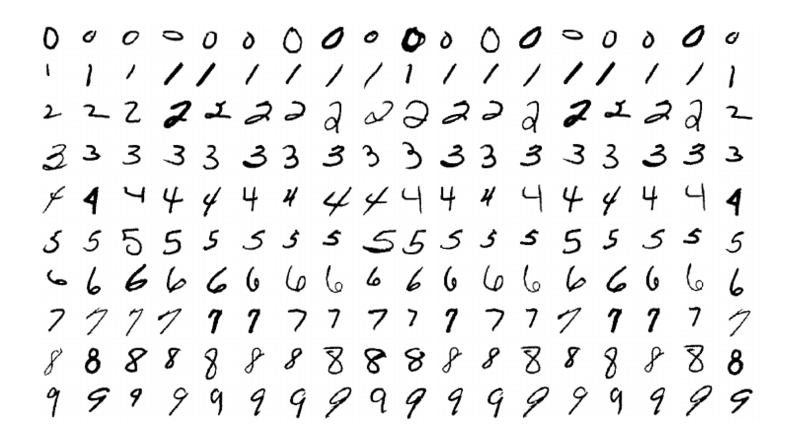
Classification Example: MNIST & LeNet-5

The MNIST dataset (Modified National Institute of Standards and Technology dataset) consists of a large collection of [math]28\times 28[/math] grayscale images of hand drawn digits. The goal is assigning to each image the correct 0-9 label.

A modernized LeNet-5 network, the classic LeNet-5 network from used sigmoidal activation functions, unusual sub-sampling layers and Gaussian connections. Replacing these with ReLUs, max pooling and fully connected layers yields a somewhat simpler network that works equally well.

General references

Smets, Bart M. N. (2024). "Mathematics of Neural Networks". arXiv:2403.04807 [cs.LG].