Deep Neural Networks

[math] \newcommand{\ul}{\mathbf} \newcommand{\symbf}{\bm} \newcommand\subsetap{\mathrel{\overset{\makebox[0pt]{\mbox{\normalfont\tiny\sffamily ap.}}}{\rule{0pt}{.8ex}\smash{\subset}}}} \newcommand{\rident}[1]{\mathrm{#1}} \newcommand{\iident}[1]{\mathit{#1}} \newcommand{\wip}{\emoji{construction}} \newcommand{\pointright}{\emoji{backhand-index-pointing-right-light-skin-tone}} \DeclareMathOperator*{\argmax}{arg\,max} \DeclareMathOperator*{\argmin}{arg\,min} \DeclareMathOperator*{\Arg}{Arg} \DeclareMathOperator*{\Var}{Var} \DeclareMathOperator*{\dom}{dom} \DeclareMathOperator{\Div}{div} \DeclareMathOperator{\morph}{\scalebox{0.7}{\ensuremath\square}} \DeclareMathOperator*{\esssup}{ess\,sup} \DeclareMathOperator{\Int}{Int} \DeclareMathOperator{\Cl}{Cl} \DeclareMathOperator{\id}{id} \DeclareMathOperator{\diam}{diam} \DeclareMathOperator{\supp}{supp} \DeclareMathOperator{\arctantwo}{arctan2} \DeclareMathOperator{\relu}{ReLU} \newcommand{\mathds}{\mathbb}[/math]

This article was automatically generated from a tex file and may contain conversion errors. If permitted, you may login and edit this article to improve the conversion.

Feed Forward Networks

The quintessential example of a deep neural network is the feed forward neural network wherein connections between nodes do not form cycles. A feed forward network simply takes a set of shallow networks and concatenates them, feeding the output of one layer of neurons as input into the next layer of neurons. Let us formalize this construction. Let [math]L \in \mathbb{N}[/math] and [math]N_0,N_1,\ldots,N_{L+1} \in \mathbb{N}[/math]. Let [math]\sigma_1,\ldots,\sigma_L[/math] be activation functions, which we will assume to be scalar functions that we apply pointwise for the moment. Let [math]F_i : \mathbb{R}^{N_{i-1}} \to \mathbb{R}^{N_i}[/math] be affine transforms given by

[[math]] \begin{equation*} F_i (\boldsymbol{x}) := A_i \boldsymbol{x} + \boldsymbol{b}_i \end{equation*} [[/math]]

where [math]A_i \in \mathbb{R}^{N_i \times N_{i-1}}[/math] and [math]\boldsymbol{b}_i \in \mathbb{R}^{N_i}[/math] for [math]i \in \{ 1, \ldots, L+1\}[/math]. Then we call [math]\mathcal{N} : \mathbb{R}^{N_0} \to \mathbb{R}^{N_{L+1}}[/math] given by

[[math]] \begin{equation} \label{eq:feedforward} \mathcal{N} := F_{L+1} \circ \sigma_L \circ F_L \circ \cdots \circ \sigma_1 \circ F_1 \end{equation} [[/math]]

a feed forward neural network. This network is said to have [math]L[/math] (hidden) layers, [math]N_i[/math] is said to be the width of the layer [math]i[/math] and the maximum of all the layer's widths, i.e. [math]\max_{i=1}^L \{ N_i \}[/math], is also called the width of the network. We usually label inputs with [math]\boldsymbol{x}[/math], outputs with [math]\boldsymbol{y}[/math] and if necessary the intermediate results with [math]\boldsymbol{z}^{(i)} \in \mathbb{R}^{N_i}[/math] as follows:

[[math]] \begin{equation*} \boldsymbol{z}^{(0)} := \boldsymbol{x} , \qquad \boldsymbol{z}^{(i)} := \sigma_i \left( F_i(\boldsymbol{z}^{(i-1)}) \right) , \end{equation*} [[/math]]

for [math]i \in \{ 1,\ldots, L+1\}[/math]. Variants to this architecture are still called feed forward networks. For example we could include multi-variate activation functions such as soft-max or max pooling, this would require us to specify the input and output widths of the layers differently but we could still write the network down as in \ref{eq:feedforward}. Another common feature is a skip connection: some of the outputs of a layer are passed to layers deeper down rather than (or in addition) to the next layer. An example of a feed forward network is illustrated in graph form in Figure figure.

Graph representation of a feed forward neural network with 3 hidden layers. Each node is computed as the activation function applied to an affine combination of its inputs. Passing signals to deeper layers rather than the next layer is also a common feature of these types of networks and is called a skip connection.

[Recurrent neural networks]

The other major class of neural networks besides feed forward are the recurrent neural networks, these networks allow for cycles to be present in their graphs. Recurrent neural networks are mainly used for processing sequential data such as in speech and natural language applications. See for a survey.

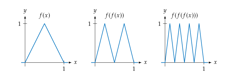
Previously we saw how a shallow neural network with ReLU activation functions results in a piecewise linear function. If we want to model a more complex function we needed to increase the width of the network, the number of linear pieces would scale linearly with the amount of neurons. Consider a sawtooth function as in Figure figure, if we wanted to model a sawtooth with [math]n[/math] teeth with a shallow ReLU network we would need [math]2 n[/math] neurons. But consider the network for [math]1[/math] tooth:

[[math]] \begin{equation} \label{eq:sawtooth} f(x) := \relu(2 x) - \relu(4 x - 2) + \relu(2 x - 2) , \end{equation} [[/math]]

and concatenate it multiple times: we would also get a more and more complex sawtooth for every concatenation as is shown in Figure figure.

Iterative application of the function [math]f[/math] from \ref{eq:sawtooth} causes an exponential increase in the complexity of the result as measured by the amount of linear pieces.

In fact we would get a doubling of the number of teeth every time we reapply [math]f[/math] and so an exponential increase in the amount of linear pieces in the output. This is the major benefit of depth: the complexity of the functions a network can model grows faster with depth than with width. This is not to say that we should design our networks with maximum depth and minimum width. As is usually the case in engineering there are tradeoffs to consider and any real network strikes a balance between width and depth.

While in a shallow ReLU network each linear piece is independent in a deep ReLU network this is not the case. This can be understood by considering that the number of parameters in a deep ReLU network scales linearly with the number of layers while the number of pieces of the output scales exponentially, at some point there will not be enough parameters to describe any piecewise linear function with that amount of pieces. With an equivalent shallow ReLU network the output space is exactly the space of all piecewise linear functions with that amount of pieces.

Vanishing and Exploding Gradients

One difficulty that arises with deep networks is in training. A parameter in an early layer of the network, it has to pass through many layers before finally contributing to the loss. Let us disregard the affine transforms of a network for the moment and focus on the activation functions. Let [math]\sigma[/math] be the sigmoid activation function given by [math]\sigma(a):=\frac{1}{1+e^{-a}}[/math], then define

[[math]] \begin{equation*} \sigma^N := \underbrace{\sigma \circ \sigma \circ \cdots \circ \sigma}_{N}. \end{equation*} [[/math]]

For computing the derivative of [math]\sigma^N[/math] we apply the chain rule to find the recursion

[[math]] \begin{equation*} \frac{\partial}{\partial a} \sigma^N (x) = \sigma' \left( \sigma^{N-1}(a) \right) \, \frac{\partial}{\partial x} \sigma^{N-1}(a). \end{equation*} [[/math]]

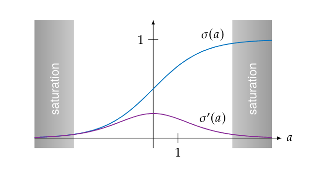
From Figure figure we deduce that [math]0 \lt \sigma'(a) \leq \frac{1}{4}[/math] so

[[math]] \begin{equation*} \left| \frac{\partial}{\partial a} \sigma^N(a) \right| \leq \left( \frac{1}{4} \right)^N . \end{equation*} [[/math]]

Consequently performing a gradient descent step of the form

[[math]] \begin{equation*} a_{i+1} = a_i - \eta \, \frac{\partial}{\partial a} \sigma^N (a_i) , \end{equation*} [[/math]]

would not change the parameter very much, a problem which becomes worse with every additional layer. Worse is that [math]\sigma'(a)[/math] goes to zero quickly for large absolute values of [math]a[/math], as can be seen in Figure figure. In this regime, when [math]\sigma(a)[/math] is close to [math]0[/math] or [math]1[/math], we say the sigmoid is saturated.

The sigmoid activation function and its derivative. Observe that the derivative is at most [math]\frac{1}{4}[/math] and goes to zero quickly as [math]a \to \pm\infty[/math], this is called saturation.

Theoretically we could train for longer to compensate for very small gradients but in practice this also does not work because of how floating point math works. Specifically when working with floating point numbers we have

[[math]] \begin{equation*} a + b = a \quad \text{if} \quad |b| \ll |a|, \end{equation*} [[/math]]

hence a small enough update to a parameter does not actually change the parameter.

This behaviour of gradients becoming smaller and smaller the deeper the network becomes is called the vanishing gradient problem. The opposite phenomenon can also occur where the gradients become larger and larger leading to unstable training, this is called the exploding gradient problem.

We can contrast the behaviour of the sigmoid with the rectified linear unit in the same situation. Recall that the ReLU is defined as [math]\relu(x):=\max\{0,x\}[/math], then we define

[[math]] \begin{equation*} \relu^N := \underbrace{\relu \circ \relu \circ \cdots \circ \relu}_{N}. \end{equation*} [[/math]]

Calculating the derivative we get:

[[math]] \begin{equation} \label{eq:relun_deriv} \frac{\partial}{\partial a} \relu^N (a) = \begin{cases} \ 1 \quad &\text{if } a \gt 0, \\ \ 0 &\text{else}, \end{cases} \end{equation} [[/math]]

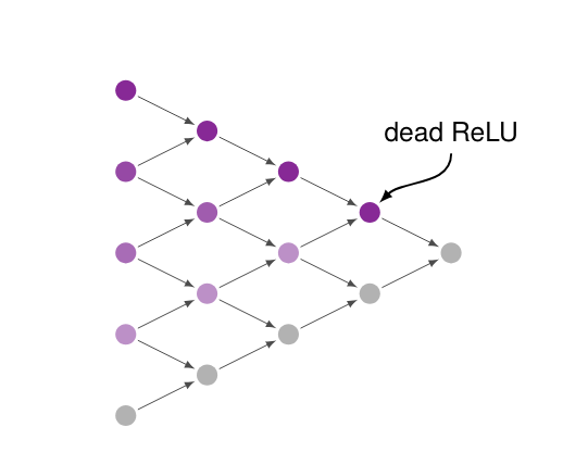
which does not depend on the number of layers [math]N[/math]. Conceptually \ref{eq:relun_deriv} can be interpreted as a ReLU allowing for a [math]1[/math] derivative for parameters that are currently affecting the loss (regardless of which layer the parameter resides in) and giving a zero derivative for parameters that do not. The ReLU (at least partially) sidestepping the vanishing/exploding gradient problem accounts for their popularity in deep neural networks. This is not to say that ReLUs are without issues. If an input to a ReLU is negative it will have a gradient of zero, we say the ReLU or the neuron is dead. Consequently all neurons in the previous layer that only (or predominantly) feed into that neuron will also have a gradient of zero (or close to zero). You could visualize this phenomenon as a dead neuron casting a shadow on the lower layers as is illustrated in Figure figure.

A dead ReLU (i.e. with negative argument and so zero derivative) will cause the gradients of the upstream neurons to also become zero, this effect will cascade all the way through to the start of the network. Neurons that feed into non-dead ReLUs will still have a gradient via those live connections. The purple shading of the nodes indicates the degree to which each node is affected by the dead ReLU.

During training, which neurons are dead and where the shadow is cast changes from batch to batch. As long as most neurons are not perpetually in the shadow we should be able to properly train the network. However, if we happen to get an unlucky initialization it is quite possible that a large part of our network is permanently stuck with zero gradients, this phenomenon is called the dying ReLU problem. Of course, the choice of activation function is not the only thing we need to consider. The gradients in a real network also depend on the current values of the parameters of the affine transforms. So we still need to initialize those parameters to values that do not cause vanishing or exploding gradient problem right from the start. We will get back to parameter initialization later on.

Scaling to High Dimensional Data

If we consider all components of a matrix [math]A_i[/math] from \ref{eq:feedforward} to be trainable parameters then we say layer [math]i[/math] is fully connected or dense, meaning all outputs of the layer depend on all inputs. When all layers are fully connected we say that the network is fully connected. Having all components of the matrices [math]A_i[/math] and vectors [math]\boldsymbol{b}_i[/math] as trainable parameters is of course not required. In fact the general fully connected feed forward network from \ref{eq:feedforward} is not often used in practice, but many architectures are specializations of this type adapted to specific applications. Specialization in this context primarily means choosing which components of the [math]A_i[/math]'s and [math]\boldsymbol{b}_i[/math]'s are trainable and which are fixed to some chosen constant. The primary reason fully connected network are not used is that they simply do not scale to high-dimensional data. Consider an application where we want to apply a transform on a [math]1000 \times 1000[/math] color image. The input and output would be elements of the space [math]\mathbb{R}^{3 \times 1000 \times 1000}[/math], a linear transform in that space would be given by a matrix

[[math]] \begin{equation*} A \in \left( \mathbb{R}^{3 \times 1000 \times 1000} \right)^2 . \end{equation*} [[/math]]

This matrix has [math]9 \cdot 10^{12}[/math] components. Storing that many numbers in 32-bit floating point format would take a whopping 36 terabytes, and that is just a single matrix. Clearly this rules out fully connected networks for high dimensional applications such as imaging. There are 3 strategies employed to deal with this problem:

• sparsity,
• weight sharing,
• parameterization.

Sparsity mean employing sparse matrices for the linear operations. When we fix most entries of a matrix to zero we do not need to store those entries and we simplify the calculation that we need to perform since we already know the result of the zeroed out parts. With weight sharing the same parameter is reused at multiple locations in the matrix. In this case we just have to store the unique parameters and not the whole matrix. Weight sharing is technically a special case of the last strategy. With parameterization we let the components of the matrix depend on a (small) number of parameter. In this case we store the parameters and compute the matrix components when required.

The following matrices are an example comparing the fully connected case with the three proposed strategies:

[[math]] \begin{equation*} \underset{ \strut \textsf{(fully connected)} } { \begin{bmatrix} a & b & c \\ d & e & f \\ g & h & i \end{bmatrix} } , \qquad \underset{ \strut \textsf{(sparse)} } { \begin{bmatrix} a & & \\ & & \\ & b & \hphantom{b} \end{bmatrix} } , \qquad \underset{ \strut \textsf{(shared weights)} } { \begin{bmatrix} a & b & b \\ b & a & b \\ b & b & a \end{bmatrix} } , \qquad \underset{ \strut \textsf{(parametrized)} } { \begin{bmatrix} f_{1}(a,b) & f_{2}(a,b) & f_{3}(a,b) \\ f_{4}(a,b) & f_{5}(a,b) & f_{6}(a,b) \\ f_{7}(a,b) & f_{8}(a,b) & f_{9}(a,b) \end{bmatrix} } , \end{equation*} [[/math]]

we need to store 9 numbers for the fully connected matrix but only 2 numbers for each of the other matrices. These 3 strategies are not mutually exclusive and we will look at an architecture that uses a combination of sparsity and weight sharing later on.

General references

Smets, Bart M. N. (2024). "Mathematics of Neural Networks". arXiv:2403.04807 [cs.LG].