Building a Rotation-translation Equivariant CNN

[math] \newcommand{\ul}{\mathbf} \newcommand{\symbf}{\bm} \newcommand\subsetap{\mathrel{\overset{\makebox[0pt]{\mbox{\normalfont\tiny\sffamily ap.}}}{\rule{0pt}{.8ex}\smash{\subset}}}} \newcommand{\rident}[1]{\mathrm{#1}} \newcommand{\iident}[1]{\mathit{#1}} \newcommand{\wip}{\emoji{construction}} \newcommand{\pointright}{\emoji{backhand-index-pointing-right-light-skin-tone}} \DeclareMathOperator*{\argmax}{arg\,max} \DeclareMathOperator*{\argmin}{arg\,min} \DeclareMathOperator*{\Arg}{Arg} \DeclareMathOperator*{\Var}{Var} \DeclareMathOperator*{\dom}{dom} \DeclareMathOperator{\Div}{div} \DeclareMathOperator{\morph}{\scalebox{0.7}{\ensuremath\square}} \DeclareMathOperator*{\esssup}{ess\,sup} \DeclareMathOperator{\Int}{Int} \DeclareMathOperator{\Cl}{Cl} \DeclareMathOperator{\id}{id} \DeclareMathOperator{\diam}{diam} \DeclareMathOperator{\supp}{supp} \DeclareMathOperator{\arctantwo}{arctan2} \DeclareMathOperator{\relu}{ReLU} \newcommand{\mathds}{\mathbb}[/math]

This article was automatically generated from a tex file and may contain conversion errors. If permitted, you may login and edit this article to improve the conversion.

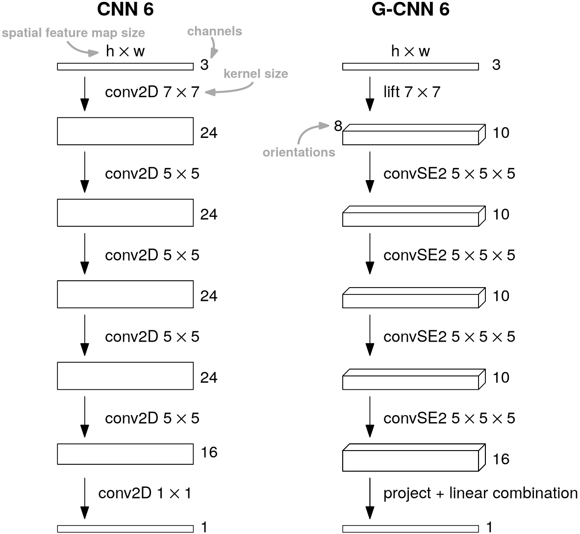
How do we now use this framework to construct a rotation-translation invariant network for images? From Example~example we know that we do not have a lot of freedom in training a rotation-translation equivariant operator from [math]\mathbb{R}^2[/math] to [math]\mathbb{R}^2[/math]. We can buy ourselves a lot more freedom by making the first linear operation in our network one that maps functions on [math]\mathbb{R}^2[/math] to functions on [math]\iident{SE}(2)[/math]. In the context of image analysis the process of transforming an image to a higher dimensional representation is called lifting. Therefore we will call the first layer in our network the lifting layer. Once we are operating on the group we have much more freedom since group convolution is equivariant. Just like in a conventional CNN we can have a series of group convolution layers that make up the bulk of our network. Of course we might not want our final product to live on the group, we might want to go back to [math]\mathbb{R}^2[/math], but we also have a recipe for that. Since going from the 3 dimensional space [math]\iident{SE}(2)[/math] to the 2 dimensional space [math]\mathbb{R}^2[/math] is akin to projection we call a layer that does this a projection layer. This three stage design is illustrated in Figure figure for the retinal vessel segmentation application. For some more examples of the use of this type of network in medical imaging applications see .

A G-CNN for retinal vessel segmentation that is rotation-translation equivariant. Lifting data to a higher dimensional space affords us more freedom in the kernels we train while maintaining equivariance.

Lifting Layer

Let [math]G=\iident{SE}(2) \equiv \mathbb{R}^2 \rtimes [0, 2\pi)[/math] using the parameterization from Example example. Let [math]M=\mathbb{R}^2[/math] and [math]N=G[/math]. Choose [math]e=(\boldsymbol{0},0) \in N[/math] as the reference element then the stabilizer [math]G_e[/math] is trivially [math]\{e\}[/math], so any kernel on [math]M=\mathbb{R}^2[/math] is compatible. The Lebesgue measure is rotation-translation equivariant so we have an invariant integral. Let [math]n_0 \in \{ 1,3 \}[/math] be the number of input channels and denote the input functions as [math]f^{(0)}_{j}:\mathbb{R}^2 \to \mathbb{R}[/math] for [math]j[/math] from [math]1[/math] to [math]n_0[/math]. Let us denote the number of desired feature maps in the first layers as [math]n_1[/math]. Recall that there are two conventions for convolution layers: single channel and multi channel. In the multi channel setup we associate with each output channel a number of kernels equal to the amount of input channels. Our parameters would be a set [math]\{ \kappa^{(1)}_{ij}\}_{ij} \subset C(\mathbb{R}^2) \cap L^1(\mathbb{R}^2)[/math] of kernels and a set [math]\{ b^{(1)}_i \}_{i} \subset \mathbb{R}[/math] of biases for [math]i[/math] from [math]1[/math] to [math]n_1[/math] and [math]j[/math] from [math]1[/math] to [math]n_0[/math]. The calculation for output channel [math]i[/math] is then given by

[[math]] \begin{equation*} f^{(1)}_{i}(\boldsymbol{x},\theta) = \sigma \left( \sum_{j=1}^{n_0} \int_{\mathbb{R}^2} \left( (\boldsymbol{x},\theta) \cdot \kappa^{(1)}_{ij}\right) (\boldsymbol{y}) \, f^{(0)}_{j}(\boldsymbol{y}) \, d \boldsymbol{y} + b^{(1)}_{i} \right) , \end{equation*} [[/math]]

for some choice of activation function [math]\sigma[/math]. In the single channel setup we associate a kernel with each input channel and then make linear combinations of the convolved input channels to generate output channels. Our parameters would then consist of a set of kernels [math]\{ \kappa^{(1)}_{j} \}_{j} \subset C(\mathbb{R}^2) \cap L^1(\mathbb{R}^2)[/math] and a set of weights [math]\{ a^{(1)}_{ij} \}_{ij} \subset \mathbb{R}[/math] and biases [math]\{ b^{(1)}_i \}_{i} \subset \mathbb{R}[/math] for [math]i[/math] from [math]1[/math] to [math]n_1[/math] and [math]j[/math] from [math]1[/math] to [math]n_0[/math]. The calculation for output channel [math]i[/math] is then given by

[[math]] \begin{equation*} f^{(1)}_{i}(\boldsymbol{x},\theta) = \sigma \left( \sum_{j=1}^{n_0} a^{(1)}_{ij} \int_{\mathbb{R}^2} \left( (\boldsymbol{x},\theta) \cdot \kappa^{(1)}_{j} \right)(\boldsymbol{y}) \, f^{(0)}_{j}(\boldsymbol{y}) \, d\boldsymbol{y} + b^{(1)}_{i} \right) . \end{equation*} [[/math]]

In either case the actual lifting happens by translating and rotating the kernel over the image, a particular translation and rotation gives us a particular scalar value at the corresponding location in [math]\iident{SE}(2)[/math].

[Orientation score transform]

If you followed the course Differential Geometry for Image Processing (2MMA70) this will seem very familiar to you. Indeed this an orientation score transform except we do not design the wavelet filter (the kernel) ourselves but leave it up to the network to train.

Group Convolution Layer

We already saw in Example example how to do convolution on the group itself. On the Lie group we always have an invariant integral (the left Haar integral) and the symmetry requirement on the kernel is trivial so we have no restrictions to take into account for training the kernel (unlike for the case [math]\mathbb{R}^2 \to \mathbb{R}^2[/math]). In layer [math]\ell \in \mathbb{N}[/math] with [math]n_{\ell-1}[/math] input channels and [math]n_{\ell}[/math] output channels the calculation for output channel [math]i[/math] is given (for the single channel setup) by

[[math]] \begin{equation*} f^{(\ell)}_{i} = \sigma \left( \sum_{j=1}^{n_{\ell-1}} a^{(\ell)}_{ij} \left( \kappa^{(\ell)}_{j} \star_G f^{(\ell-1)}_{j} \right) + b^{(\ell)}_{i} \right) \end{equation*} [[/math]]

for all [math]i \in \{1, \ldots, n_{\ell} \}[/math] or

[[math]] \begin{equation*} f^{(\ell)}_{i} (\boldsymbol{x},\theta) = \sigma \left( \sum_{j=1}^{n_{\ell}} a^{(\ell)}_{ij} \int_{\mathbb{R}^2} \int_{0}^{2\pi} \left( (\boldsymbol{x},\theta) \cdot \kappa^{(\ell)}_{j} \right) (\boldsymbol{y},\alpha) \ f^{(\ell-1)}_{j}(\boldsymbol{y},\alpha) \ d\alpha d\boldsymbol{y} + b^{(\ell)}_{i} \right) , \end{equation*} [[/math]]

for some choice of activation function [math]\sigma[/math]. Here the kernels [math]\kappa^{(\ell)}_{j} \in C(G)\times L^1(G)[/math], the weights [math]a^{(\ell)}_{i j} \in \mathbb{R}[/math] and the biases [math]b^{(\ell)}_i \in \mathbb{R}[/math] are the trainable parameters. Deducing the formula for the multi channel setup we leave as an exercise.

Group convolution layers can be stacked sequentially just like normal convolution layers in a CNN to make up the heart of a G-CNN, see Figure figure.

Projection

The desired output of our network is likely not a feature map on the group or some other higher dimensional homogeneous space. So at some point we have to transition away from them. In traditional CNNs used for classification we saw that at some point we flattened our multi-dimensional array by `forgetting' the spatial dimensions. Once we have discretized, flattening is of course also a viable approach for a G-CNN when the goal is classification. However we might not want to throw away our spatial structure, if the goal of the network is to transform its input in some way then we want to go back to our original input space (like in the example in Figure figure). Applying our equivariance framework again to the case [math]G=M=\iident{SE}(2)[/math] and [math]N=\mathbb{R}^2[/math]. Choose [math]\boldsymbol{0} \in N[/math] as the reference element then its stabilizer is the subgroup of just rotations. So to construct an equivariant linear operator from [math]\iident{SE}(2)[/math] to [math]\mathbb{R}^2[/math] requires a kernel [math]\kappa[/math] on [math]\iident{SE}(2)[/math] that satisfies

[[math]] \begin{equation*} (\boldsymbol{0},\, \beta) \cdot \kappa = \kappa \quad\Leftrightarrow\quad \kappa(\boldsymbol{x},\,\theta) = \kappa\left( R(-\beta) \boldsymbol{x},\, \theta - \beta \right) \qquad \forall \beta,\theta \in [0,2\pi),\, \boldsymbol{x} \in \mathbb{R}^2 , \end{equation*} [[/math]]

where [math]R(-\theta)[/math] is the rotation matrix over [math]-\theta[/math]. Consequently we can reduce the trainable (unrestricted) part of the kernel [math]\kappa[/math] to a 2 dimensional slice:

[[math]] \begin{equation*} \kappa(\boldsymbol{x},\theta) = \kappa\left( R(-\theta)\boldsymbol{x},\, 0 \right) . \end{equation*} [[/math]]

A kernel like this gives us the desired equivariant linear operator and with a set of them we can construct a layer in the same fashion as the lifting and group convolution layer.

In practice this type of operator with trainable kernel is not what is used for projection from [math]\iident{SE}(2)[/math] to [math]\mathbb{R}^2[/math]. Instead the much simpler (and non-trainable) integration over the [math]\theta[/math] axis is used, let [math]f \in \iident{B}(\iident{SE}(2))[/math] then the operator [math]P:C(\iident{SE}(2)) \cap B(\iident{SE}(2)) \to C(\mathbb{R}^2) \cap B(\mathbb{R}^2)[/math] given by

[[math]] \begin{equation} \label{eq:integration_over_theta} (Pf)(\boldsymbol{x}) := \int_{0}^{2\pi} f(\boldsymbol{x},\theta) \, d\theta, \end{equation} [[/math]]

is a bounded linear operator that is rotation-translation equivariant.

Note that the projection operator \ref{eq:integration_over_theta} is one of our equivariant linear operators if we take the kernel to be [math]\kappa_P(\boldsymbol{x},\theta)=\delta(\boldsymbol{x})[/math] where [math]\delta[/math] is the Dirac delta on [math]\mathbb{R}^2[/math]. The Dirac delta is not a function in [math]C(G) \cap L^1(G)[/math] but we can take a sequence in [math]C(G) \cap L^1(G)[/math] that has [math]\kappa_P[/math] as the limit in the weak sense, such as a sequence of narrowing Gaussians.

A common alternative to integrating over the orientation axis is taking the maximum over that axis:

[[math]] \begin{equation} \label{eq:max_projection_layer} \left( P_{\max} f \right)(\boldsymbol{x}) := \max_{\theta \in [0,2\pi)} \, f(\boldsymbol{x},\theta). \end{equation} [[/math]]

This is not a linear operator but it is rotation-translation equivariant, we will revisit this projection operator later. After we have once again obtained feature maps on [math]\mathbb{R}^2[/math] we can proceed to our desired output format in the same way as we would do with a classic CNN. Either we forget the spatial dimensions and transition to a fully connected network for classification applications or we take a linear combination of the obtained 2D feature maps to generate an output image such as in Figure figure and .

Discretization

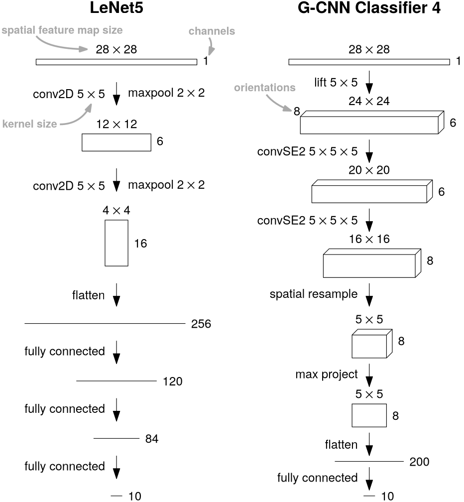
To implement our developed G-CNN in practice we will need to switch to a discretized setting. For our specific case of an [math]\iident{SE}(2)[/math] G-CNN the lifting layer typically uses kernels of size [math]5 \times 5[/math] to [math]7 \times 7[/math]. We usually choose the number of discrete orientations to be [math]8[/math], so an input of [math]\mathbb{R}^{H \times W}[/math] would be lifted to [math]\mathbb{R}^{8\times H \times W}[/math], this may seem low but empirically this is around the sweet-spot between performance and memory usage/computation time. The group convolution layers usually employ [math]5 \times 5 \times 5[/math] kernels. In both cases we need to sample the kernel off-grid to be able to rotate them, for that we almost always use linear interpolation. Example G-CNN implementations are illustrated in Figure figure for both segmentation and classification, examples for various medical applications can be found in .

A traditional CNN (left) versus a rotation-translation equivariant G-CNN (right) for segmenting a [math]h \times w[/math] color image. Figure~figure shows an application of this type.

As a general rule of thumb in deep learning we discretize as coarsely as we can get away with. Increasing the size of the kernels or the number of orientations does increase performance but nowhere near proportional to the increase in memory and computation time this causes. Keeping coarse kernels and increasing the depth of the network is a better way of spending a given memory/time budget.

[Linear interpolation alternatives]

Higher order polynomial interpolation methods are highly undesirable on such coarse grids, as the oscillations can make the network behave erratically. More advanced interpolation techniques have been proposed, see for example , but the added computationally complexity can be a drawback. Just as with discretization, the rule of thumb for interpolation is: as coarsely as you can get away with.

General references

Smets, Bart M. N. (2024). "Mathematics of Neural Networks". arXiv:2403.04807 [cs.LG].