Adaptive Learning Rate Algorithms

[math] \newcommand{\ul}{\mathbf} \newcommand{\symbf}{\bm} \newcommand\subsetap{\mathrel{\overset{\makebox[0pt]{\mbox{\normalfont\tiny\sffamily ap.}}}{\rule{0pt}{.8ex}\smash{\subset}}}} \newcommand{\rident}[1]{\mathrm{#1}} \newcommand{\iident}[1]{\mathit{#1}} \newcommand{\wip}{\emoji{construction}} \newcommand{\pointright}{\emoji{backhand-index-pointing-right-light-skin-tone}} \DeclareMathOperator*{\argmax}{arg\,max} \DeclareMathOperator*{\argmin}{arg\,min} \DeclareMathOperator*{\Arg}{Arg} \DeclareMathOperator*{\Var}{Var} \DeclareMathOperator*{\dom}{dom} \DeclareMathOperator{\Div}{div} \DeclareMathOperator{\morph}{\scalebox{0.7}{\ensuremath\square}} \DeclareMathOperator*{\esssup}{ess\,sup} \DeclareMathOperator{\Int}{Int} \DeclareMathOperator{\Cl}{Cl} \DeclareMathOperator{\id}{id} \DeclareMathOperator{\diam}{diam} \DeclareMathOperator{\supp}{supp} \DeclareMathOperator{\arctantwo}{arctan2} \DeclareMathOperator{\relu}{ReLU} \newcommand{\mathds}{\mathbb}[/math]

This article was automatically generated from a tex file and may contain conversion errors. If permitted, you may login and edit this article to improve the conversion.

The learning rate is crucial to the success of the training process. In general the loss is highly sensitive to some parameters but insensitive to others, just think about parameters in different layers. Momentum alleviates some of the issues but introduces problems of its own and adds another hyperparameter we have to tune. Assigning each parameters its own learning rate (and continually adjusting it) is not feasible. What we need are automatic methods. This has lead to the development of adaptive learning (rate) algorithms. The idea is to set the learning rate dynamically per-parameter at each iteration based on the history of the gradients. We will look at three of these methods: Adagrad, RMSProp and Adam. Let us recall the setting. We have a parameter space [math]W = \mathbb{R}^N[/math] and some initial parameter value [math]w_0 \in W[/math]. Let [math]I_t[/math] be the batch at iteration [math]t \in \mathbb{N}[/math] and [math]\ell_{I_t}[/math] its associated loss function. We will abbreviate the current batch's gradient as:

[[math]] \begin{equation*} g_t := \nabla \ell_{I_t} (w_t). \end{equation*} [[/math]]

The SGD update rule with learning rate [math]\eta \gt 0[/math] is then:

[[math]] \begin{equation*} w_{t+1} = w_t - \eta g_t . \end{equation*} [[/math]]

With momentum the update rule becomes:

[[math]] \begin{equation*} \begin{split} v_{t} &= \mu v_{t-1} - \eta g_t, \\ w_{t+1} &= w_t + v_t, \end{split} \end{equation*} [[/math]]

where [math]v_0 = 0[/math] and [math]\mu \in [0,1)[/math] is the momentum factor.

Adagrad

Adagrad (Adaptive Gradient Descent) was one of the first adaptive learning rate methods introduced by . Let [math]t \in \mathbb{N}_0[/math], [math]I_t[/math] the batch index set at iteration [math]t[/math] and [math]\ell_{I_t}[/math] its associated loss. Let [math]w_0[/math] be the initial parameter values and abbreviate [math]g_t := \nabla \ell_{I_t}(w_t)[/math]. The Adagrad update is defined per-parameter as:

[[math]] \begin{equation*} \left( w_{t+1} \right)_i = \left( w_t \right)_i - \frac{\eta}{\sqrt{\sum_{k=0}^t \left( g_k \right)_i^2} + \varepsilon} \left( g_t \right)_i . \end{equation*} [[/math]]

Or when we take all the operations on the vectors to mean component-wise operations we can write more concisely:

[[math]] \begin{equation*} w_{t+1} = w_t - \frac{\eta}{\sqrt{\sum_{k=0}^t g_k^2 } + \varepsilon} g_t . \end{equation*} [[/math]]

At each iterations we slow down the effective learning rate of each individual parameter by the [math]L^2[/math] norm of the history of the partial derivatives with respect to that parameter. As [math](g_t)_i[/math] may be very small or zero we add a small positive [math]\varepsilon[/math] (say [math]10^{-8}[/math] or so) for numerical stability. The benefit of this method is that choosing [math]\eta[/math] becomes less important, the step size will eventually decrease to the point that it can settle into a local minimum. On the other hand, the denominator [math]\sqrt{\sum_{k=0}^t \left( g_k \right)_i^2}[/math] is monotonically decreasing and will eventually bring the training process to a halt whether a local minimum has been reach or not.

RMSProp

Root Mean Square Propagation or RMSProp is an adaptive learning rate algorithm introduced by . RMSProp uses the same basic idea as Adagrad, but instead of accumulating the squared gradients it uses a weighted average of the historic gradients. Let [math]\alpha \in (0,1)[/math]:

[[math]] \begin{equation*} \begin{split} v_{t} &= \alpha v_{t-1} + (1-\alpha) g_t^2 \\ w_{t+1} &= w_t - \frac{\eta}{\sqrt{v_t} + \varepsilon} g_t, \end{split} \end{equation*} [[/math]]

where again all the arithmetic operations are applied component-wise. The [math]\alpha[/math] factor is called the forgetting factor, decay rate or smoothing factor. The suggested hyperparameter values to start with are [math]\eta=0.001[/math] and [math]\alpha=0.9[/math].

Adam

The Adaptive Moment Estimation method, or Adam, was introduced by . In addition to storing an exponentially decaying average of past square gradients [math]v_t[/math] like RMSProp, Adam also keeps a running average of past gradients [math]m_t[/math], similar to momentum. Let [math]\beta_1, \beta_1 \in (0,1)[/math],

[[math]] \begin{equation*} \begin{split} m_{t} &= \beta_1 m_{t-1} + (1-\beta_1) g_t , \\ v_{t} &= \beta_2 v_{t-1} + (1-\beta_2) (g_t)^2 , \end{split} \end{equation*} [[/math]]

with [math]m_0 = v_0 = 0[/math]. The vectors [math]m_t[/math] and [math]v_t[/math] are estimates of the first moment (the mean) and the second moment (the uncentered variance), hence the name of the method. As we start with [math]m_0 = v_0 =0[/math] the estimates are biased towards zero. Let us see how biased and whether we can correct that bias. By induction we have:

[[math]] \begin{equation*} \begin{split} m_t &= (1-\beta_1) \sum_{i=1}^t \beta_1^{t-i} g_i, \\ v_t &= (1-\beta_2) \sum_{i=1}^t \beta_2^{t-i} (g_i)^2, \end{split} \end{equation*} [[/math]]

and so:

[[math]] \begin{equation*} \begin{split} \mathbb{E}[m_t] &= (1-\beta_1) \sum_{i=1}^t \beta_1^{t-i} \mathbb{E}[g_i], \\ \mathbb{E}[v_t] &= (1-\beta_2) \sum_{i=1}^t \beta_2^{t-i} \mathbb{E}[(g_i)^2]. \end{split} \end{equation*} [[/math]]

Assuming [math]\mathbb{E}[g_i][/math] and [math] \mathbb{E}[(g_i)^2][/math] are stationary (i.e. do not depend on [math]i[/math]) we get:

[[math]] \begin{equation*} \begin{split} \mathbb{E}[m_t] &= \left((1-\beta_1) \sum_{i=1}^t \beta_1^{t-i}\right) \mathbb{E}[g_t], \\ \mathbb{E}[v_t] &= \left((1-\beta_2) \sum_{i=1}^t \beta_2^{t-i} \right) \mathbb{E}[(g_t)^2]. \end{split} \end{equation*} [[/math]]

Which simplifies to:

[[math]] \begin{equation*} \begin{split} \mathbb{E}[m_t] &= (1-\beta_1^t) \mathbb{E}[g_t], \\ \mathbb{E}[v_t] &= (1-\beta_2^t) \mathbb{E}[(g_t)^2]. \end{split} \end{equation*} [[/math]]

Therefore, the bias-corrected moments are:

[[math]] \begin{equation*} \hat{m}_t = \frac{m_t}{1-\beta_1^t} , \qquad \hat{v}_t = \frac{v_t}{1-\beta_2^t} . \end{equation*} [[/math]]

The update rule of Adam is then given by:

[[math]] \begin{equation*} w_{t+1} = w_t - \eta \frac{\hat{m}_t}{\sqrt{\hat{v}_t} + \varepsilon}, \end{equation*} [[/math]]

where again all arithmetic is applied component-wise. The default hyperparameter values suggested by are [math]\eta=0.001[/math], [math]\beta_1=0.9[/math], [math]\beta_2=0.99[/math] and [math]\varepsilon=10^{-8}[/math].

Which variant to use?

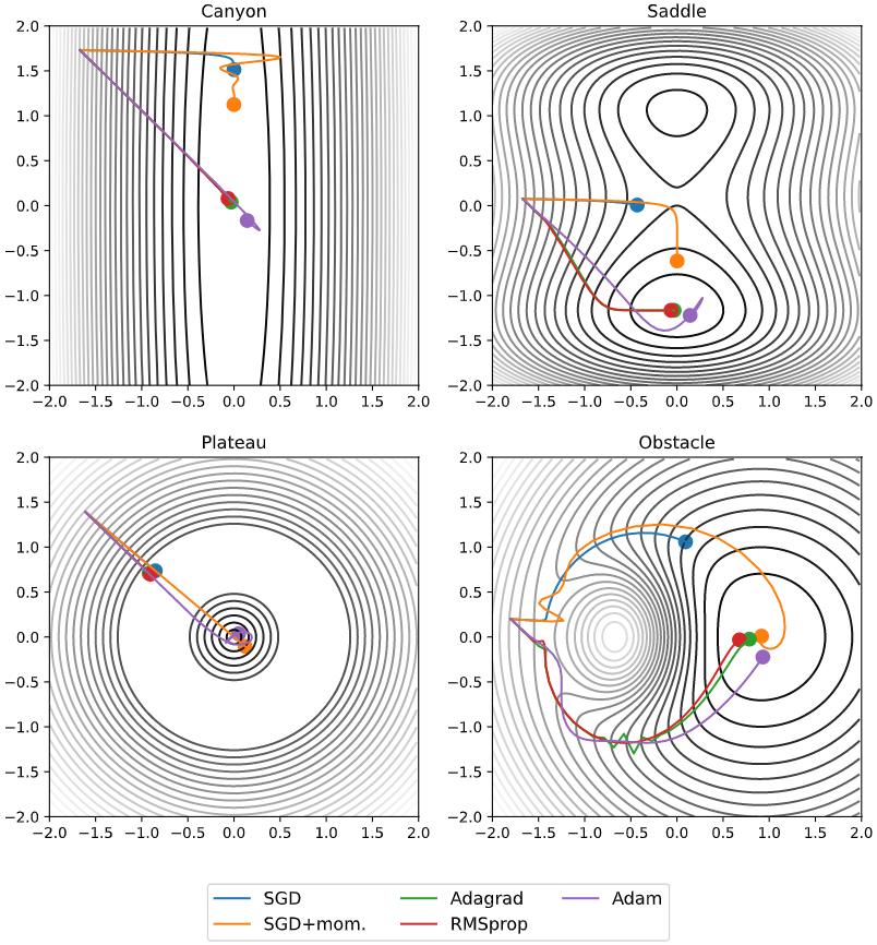
Which of these algorithms should you use? If your data is sparse (very high dimensional data usually is) then the adaptive learning rate methods usually outperform plain SGD (with or without momentum). showed that due to its bias correction Adam performs marginally better late in the training process. In that regard Adam is a safe option to try first. Nonetheless trying different algorithms to see which one works best for any given problem can be worthwhile. Fig.~figure illustrates the different behaviour of the methods we have discussed in some artificial loss landscapes. These landscapes model some of the problems the algorithms may encounter and show some of the strengths and weaknesses of each method.

Comparing 5 SGD variants in 4 different situations for a number of steps. In the canyon situation we have one parameters that has a large effect on the loss and one parameter that has little effect on the loss. The saddle situation has a prominent saddle point. The plateau has a large flat section with a vanishing gradient that needs to be traversed to get to the minimum. The final situation has an obstacle the algorithm has to go around to reach the minimum. Dark level sets indicate lower function values. This figure was generated with R.

There are many more SGD variants we have not discussed, you can look at the R namespace in the PyTorch documentation to see the available algorithms.

General references

Smets, Bart M. N. (2024). "Mathematics of Neural Networks". arXiv:2403.04807 [cs.LG].