Model Accuracy Assessment

Mean Squared Error

In statistics, the mean squared error (MSE) or mean squared deviation (MSD) of an estimator (of a procedure for estimating an unobserved quantity) measures the average of the squares of the errors—that is, the average squared difference between the estimated values and the actual value. MSE is a risk function, corresponding to the expected value of the squared error loss. The fact that MSE is almost always strictly positive (and not zero) is because of randomness or because the estimator does not account for information that could produce a more accurate estimate. In machine learning, specifically empirical risk minimization, MSE may refer to the empirical risk (the average loss on an observed data set), as an estimate of the true MSE (the true risk: the average loss on the actual population distribution).

The MSE is a measure of the quality of an estimator. As it is derived from the square of Euclidean distance, it is always a positive value that decreases as the error approaches zero.

The MSE is the second moment (about the origin) of the error, and thus incorporates both the variance of the estimator (how widely spread the estimates are from one data sample to another) and its bias (how far off the average estimated value is from the true value). For an unbiased estimator, the MSE is the variance of the estimator. Like the variance, MSE has the same units of measurement as the square of the quantity being estimated. In an analogy to standard deviation, taking the square root of MSE yields the root-mean-square error or root-mean-square deviation (RMSE or RMSD), which has the same units as the quantity being estimated; for an unbiased estimator, the RMSE is the square root of the variance, known as the standard error.

Definition and basic properties

The MSE either assesses the quality of a predictor (i.e., a function mapping arbitrary inputs to a sample of values of some random variable), or of an estimator (i.e., a mathematical function mapping a sample of data to an estimate of a parameter of the population from which the data is sampled). The definition of an MSE differs according to whether one is describing a predictor or an estimator.

Predictor

If a vector of [math]n[/math] predictions is generated from a sample of [math]n[/math] data points on all variables, and [math]Y[/math] is the vector of observed values of the variable being predicted, with [math]\hat{Y}[/math] being the predicted values (e.g. as from a least-squares fit), then the within-sample MSE of the predictor is computed as

[[math]]\operatorname{MSE}=\frac{1}{n} \sum_{i=1}^n \left(Y_i-\hat{Y_i}\right)^2.[[/math]]

In other words, the MSE is the mean [math]\left(\frac{1}{n} \sum_{i=1}^n \right)[/math] of the squares of the errors [math]\left(Y_i-\hat{Y_i}\right)^2[/math]. This is an easily computable quantity for a particular sample (and hence is sample-dependent).

In matrix notation,

[[math]]\operatorname{MSE}=\frac{1}{n}\sum_{i=1}^n(e_i)^2=\frac{1}{n}\mathbf e^\mathsf T \mathbf e[[/math]]

where [math]e_i[/math] is [math] (Y_i-\hat{Y_i}) [/math] and [math]\mathbf e[/math] is the [math] n \times 1 [/math] column vector.

The MSE can also be computed on q data points that were not used in estimating the model, either because they were held back for this purpose, or because these data have been newly obtained. Within this process, known as statistical learning, the MSE is often called the test MSE, and is computed as

[[math]]\operatorname{MSE} = \frac{1}{q} \sum_{i=n+1}^{n+q} \left(Y_i-\hat{Y_i}\right)^2.[[/math]]

Estimator

The MSE of an estimator [math]\hat{\theta}[/math] with respect to an unknown parameter [math]\theta[/math] is defined as

[[math]]\operatorname{MSE}(\hat{\theta})=\operatorname{E}_{\theta}\left[(\hat{\theta}-\theta)^2\right].[[/math]]

This definition depends on the unknown parameter, but the MSE is a priori a property of an estimator. The MSE could be a function of unknown parameters, in which case any estimator of the MSE based on estimates of these parameters would be a function of the data (and thus a random variable). If the estimator [math]\hat{\theta}[/math] is derived as a sample statistic and is used to estimate some population parameter, then the expectation is with respect to the sampling distribution of the sample statistic.

The MSE can be written as the sum of the variance of the estimator and the squared bias of the estimator, providing a useful way to calculate the MSE and implying that in the case of unbiased estimators, the MSE and variance are equivalent.

[[math]]\operatorname{MSE}(\hat{\theta})=\operatorname{Var}_{\theta}(\hat{\theta})+ \operatorname{Bias}(\hat{\theta},\theta)^2.[[/math]]

But in real modeling case, MSE could be described as the addition of model variance, model bias, and irreducible uncertainty (see Bias–variance tradeoff). According to the relationship, the MSE of the estimators could be simply used for the efficiency comparison, which includes the information of estimator variance and bias. This is called MSE criterion.

Examples

Mean

Suppose we have a random sample of size [math]n[/math] from a population, [math]X_1,\dots,X_n[/math]. Suppose the sample units were chosen with replacement. That is, the [math]n[/math] units are selected one at a time, and previously selected units are still eligible for selection for all [math]n[/math] draws. The usual estimator for the [math]\mu[/math] is the sample average

[[math]]\overline{X}=\frac{1}{n}\sum_{i=1}^n X_i [[/math]]

which has an expected value equal to the true mean [math]\mu[/math] (so it is unbiased) and a mean squared error of

[[math]]\operatorname{MSE}\left(\overline{X}\right)=\operatorname{E}\left[\left(\overline{X}-\mu\right)^2\right]=\left(\frac{\sigma}{\sqrt{n}}\right)^2= \frac{\sigma^2}{n}[[/math]]

where [math]\sigma^2[/math] is the population variance.

For a Gaussian distribution, this is the best unbiased estimator (i.e., one with the lowest MSE among all unbiased estimators), but not, say, for a uniform distribution.

Variance

The usual estimator for the variance is the corrected sample variance:

[[math]]S^2_{n-1} = \frac{1}{n-1}\sum_{i=1}^n\left(X_i-\overline{X} \right)^2 =\frac{1}{n-1}\left(\sum_{i=1}^n X_i^2-n\overline{X}^2\right).[[/math]]

This is unbiased (its expected value is [math]\sigma^2[/math]), hence also called the unbiased sample variance, and its MSE is

[[math]]\operatorname{MSE}(S^2_{n-1})= \frac{1}{n} \left(\mu_4-\frac{n-3}{n-1}\sigma^4\right) =\frac{1}{n} \left(\gamma_2+\frac{2n}{n-1}\right)\sigma^4,[[/math]]

where [math]\mu_4[/math] is the fourth central moment of the distribution or population, and [math]\gamma_2=\mu_4/\sigma^4-3[/math] is the excess kurtosis.

However, one can use other estimators for [math]\sigma^2[/math] which are proportional to [math]S^2_{n-1}[/math], and an appropriate choice can always give a lower mean squared error. If we define

[[math]]S^2_a = \frac{n-1}{a}S^2_{n-1}= \frac{1}{a}\sum_{i=1}^n\left(X_i-\overline{X}\,\right)^2[[/math]]

then we calculate:

[[math]]\begin{align*} \operatorname{MSE}(S^2_a) &=\operatorname{E}\left[\left(\frac{n-1}{a} S^2_{n-1}-\sigma^2\right)^2 \right] \\ &= \operatorname{E}\left[ \frac{(n-1)^2}{a^2} S^4_{n-1} -2 \left ( \frac{n-1}{a} S^2_{n-1} \right ) \sigma^2 + \sigma^4 \right ] \\ &= \frac{(n-1)^2}{a^2} \operatorname{E}\left[ S^4_{n-1} \right ] - 2 \left ( \frac{n-1}{a}\right ) \operatorname{E}\left[ S^2_{n-1} \right ] \sigma^2 + \sigma^4 \\ &= \frac{(n-1)^2}{a^2} \operatorname{E}\left[ S^4_{n-1} \right ] - 2 \left ( \frac{n-1}{a}\right ) \sigma^4 + \sigma^4 && \operatorname{E}\left[ S^2_{n-1} \right ] = \sigma^2 \\ &= \frac{(n-1)^2}{a^2} \left ( \frac{\gamma_2}{n} + \frac{n+1}{n-1} \right ) \sigma^4- 2 \left ( \frac{n-1}{a}\right ) \sigma^4+\sigma^4 && \operatorname{E}\left[ S^4_{n-1} \right ] = \operatorname{MSE}(S^2_{n-1}) + \sigma^4 \\ &=\frac{n-1}{n a^2} \left ((n-1)\gamma_2+n^2+n \right ) \sigma^4- 2 \left ( \frac{n-1}{a}\right ) \sigma^4+\sigma^4 \end{align*}[[/math]]

This is minimized when

[[math]]a=\frac{(n-1)\gamma_2+n^2+n}{n} = n+1+\frac{n-1}{n}\gamma_2.[[/math]]

For a Gaussian distribution, where [math]\gamma_2=0[/math], this means that the MSE is minimized when dividing the sum by [math]a=n+1[/math]. The minimum excess kurtosis is [math]\gamma_2=-2[/math], which is achieved by a Bernoulli distribution with [math]p[/math] = 1/2 (a coin flip), and the MSE is minimized for [math]a=n-1+\tfrac{2}{n}.[/math] Hence regardless of the kurtosis, we get a "better" estimate (in the sense of having a lower MSE) by scaling down the unbiased estimator a little bit; this is a simple example of a shrinkage estimator: one "shrinks" the estimator towards zero (scales down the unbiased estimator).

Further, while the corrected sample variance is the best unbiased estimator (minimum mean squared error among unbiased estimators) of variance for Gaussian distributions, if the distribution is not Gaussian, then even among unbiased estimators, the best unbiased estimator of the variance may not be [math]S^2_{n-1}.[/math]

Gaussian distribution

The following table gives several estimators of the true parameters of the population, μ and σ², for the Gaussian case.

True value	Estimator	Mean squared error
[math]\theta=\mu[/math]	[math]\hat{\theta}[/math] = the unbiased estimator of the population mean, [math]\overline{X}=\frac{1}{n}\sum_{i=1}^n(X_i)[/math]	[math]\operatorname{MSE}(\overline{X})=\operatorname{E}((\overline{X}-\mu)^2)=\left(\frac{\sigma}{\sqrt{n}}\right)^2[/math]
[math]\theta=\sigma^2[/math]	[math]\hat{\theta}[/math] = the unbiased estimator of the population variance, [math]S^2_{n-1} = \frac{1}{n-1}\sum_{i=1}^n\left(X_i-\overline{X}\,\right)^2[/math]	[math]\operatorname{MSE}(S^2_{n-1})=\operatorname{E}((S^2_{n-1}-\sigma^2)^2)=\frac{2}{n - 1}\sigma^4[/math]
[math]\theta=\sigma^2[/math]	[math]\hat{\theta}[/math] = the biased estimator of the population variance, [math]S^2_{n} = \frac{1}{n}\sum_{i=1}^n\left(X_i-\overline{X}\,\right)^2[/math]	[math]\operatorname{MSE}(S^2_{n})=\operatorname{E}((S^2_{n}-\sigma^2)^2)=\frac{2n - 1}{n^2}\sigma^4[/math]
[math]\theta=\sigma^2[/math]	[math]\hat{\theta}[/math] = the biased estimator of the population variance, [math]S^2_{n+1} = \frac{1}{n+1}\sum_{i=1}^n\left(X_i-\overline{X}\,\right)^2[/math]	[math]\operatorname{MSE}(S^2_{n+1})=\operatorname{E}((S^2_{n+1}-\sigma^2)^2)=\frac{2}{n + 1}\sigma^4[/math]

Interpretation

An MSE of zero, meaning that the estimator [math]\hat{\theta}[/math] predicts observations of the parameter [math]\theta[/math] with perfect accuracy, is ideal (but typically not possible).

Values of MSE may be used for comparative purposes. Two or more statistical models may be compared using their MSEs—as a measure of how well they explain a given set of observations: An unbiased estimator (estimated from a statistical model) with the smallest variance among all unbiased estimators is the best unbiased estimator or MVUE (Minimum-Variance Unbiased Estimator).

Both analysis of variance and linear regression techniques estimate the MSE as part of the analysis and use the estimated MSE to determine the statistical significance of the factors or predictors under study. The goal of experimental design is to construct experiments in such a way that when the observations are analyzed, the MSE is close to zero relative to the magnitude of at least one of the estimated treatment effects.

In one-way analysis of variance, MSE can be calculated by the division of the sum of squared errors and the degree of freedom. Also, the f-value is the ratio of the mean squared treatment and the MSE.

Loss function

Squared error loss is one of the most widely used loss functions in statistics, though its widespread use stems more from mathematical convenience than considerations of actual loss in applications. Carl Friedrich Gauss, who introduced the use of mean squared error, was aware of its arbitrariness and was in agreement with objections to it on these grounds. The mathematical benefits of mean squared error are particularly evident in its use at analyzing the performance of linear regression, as it allows one to partition the variation in a dataset into variation explained by the model and variation explained by randomness.

Criticism

The use of mean squared error without question has been criticized by the decision theorist James Berger. Mean squared error is the negative of the expected value of one specific utility function, the quadratic utility function, which may not be the appropriate utility function to use under a given set of circumstances. There are, however, some scenarios where mean squared error can serve as a good approximation to a loss function occurring naturally in an application.

Like variance, mean squared error has the disadvantage of heavily weighting outliers. This is a result of the squaring of each term, which effectively weights large errors more heavily than small ones. This property, undesirable in many applications, has led researchers to use alternatives such as the mean absolute error, or those based on the median.

In statistics and machine learning, the bias–variance tradeoff is the property of a model that the variance of the parameter estimated across samples can be reduced by increasing the bias in the estimated parameters. The bias–variance dilemma or bias–variance problem is the conflict in trying to simultaneously minimize these two sources of error that prevent supervised learning algorithms from generalizing beyond their training set:

• The bias error is an error from erroneous assumptions in the learning machine learning. High bias can cause an algorithm to miss the relevant relations between features and target outputs (underfitting).
• The variance is an error from sensitivity to small fluctuations in the training set. High variance may result from an algorithm modeling the random noise in the training data (overfitting).

The bias–variance decomposition is a way of analyzing a learning algorithm's expected generalization error with respect to a particular problem as a sum of three terms, the bias, variance, and a quantity called the irreducible error, resulting from noise in the problem itself.

Motivation

• 

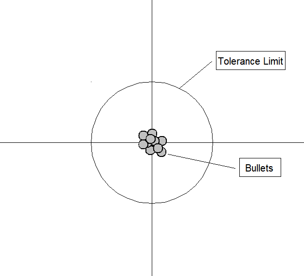
  bias low,variance low

• 

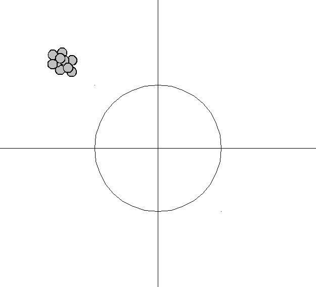
  bias high,
  variance low

• 

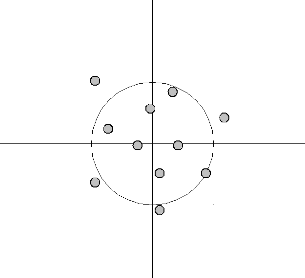
  bias low,
  variance high

• 

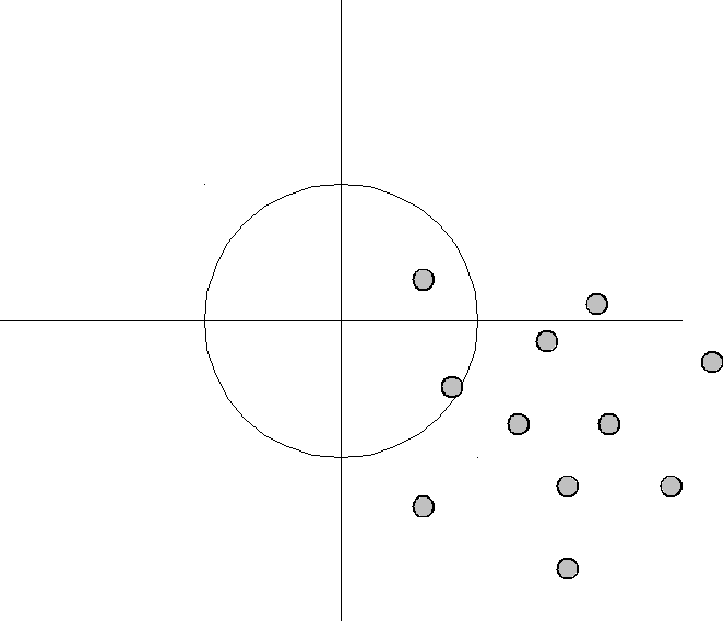
  bias high,
  variance high

The bias–variance tradeoff is a central problem in supervised learning. Ideally, one wants to choose a model that both accurately captures the regularities in its training data, but also generalizes well to unseen data. Unfortunately, it is typically impossible to do both simultaneously. High-variance learning methods may be able to represent their training set well but are at risk of overfitting to noisy or unrepresentative training data. In contrast, algorithms with high bias typically produce simpler models that may fail to capture important regularities (i.e. underfit) in the data.

It is an often made fallacy to assume that complex models must have high variance; High variance models are 'complex' in some sense, but the reverse needs not be true. In addition, one has to be careful how to define complexity: In particular, the number of parameters used to describe the model is a poor measure of complexity. This is illustrated by an example adapted from: The model

[[math]]f_{a,b}(x)=a\sin(bx)[[/math]]

has only two parameters ([math]a,b[/math]) but it can interpolate any number of points by oscillating with a high enough frequency, resulting in both a high bias and high variance.

An analogy can be made to the relationship between accuracy and precision. Accuracy is a description of bias and can intuitively be improved by selecting from only local information. Consequently, a sample will appear accurate (i.e. have low bias) under the aforementioned selection conditions, but may result in underfitting. In other words, test data may not agree as closely with training data, which would indicate imprecision and therefore inflated variance. A graphical example would be a straight line fit to data exhibiting quadratic behavior overall. Precision is a description of variance and generally can only be improved by selecting information from a comparatively larger space. The option to select many data points over a broad sample space is the ideal condition for any analysis. However, intrinsic constraints (whether physical, theoretical, computational, etc.) will always play a limiting role. The limiting case where only a finite number of data points are selected over a broad sample space may result in improved precision and lower variance overall, but may also result in an overreliance on the training data (overfitting). This means that test data would also not agree as closely with the training data, but in this case the reason is due to inaccuracy or high bias. To borrow from the previous example, the graphical representation would appear as a high-order polynomial fit to the same data exhibiting quadratic behavior. Note that error in each case is measured the same way, but the reason ascribed to the error is different depending on the balance between bias and variance. To mitigate how much information is used from neighboring observations, a model can be smoothed via explicit regularization, such as shrinkage.

Bias–variance decomposition of mean squared error

Suppose that we have a training set consisting of a set of points [math]x_1, \dots, x_n[/math] and real values [math]y_i[/math] associated with each point [math]x_i[/math]. We assume that there is a function with noise [math]y = f(x) + \varepsilon[/math], where the noise, [math]\varepsilon[/math], has zero mean and variance [math]\sigma^2[/math].

We want to find a function [math]\hat{f}(x;D)[/math], that approximates the true function [math]f(x)[/math] as well as possible, by means of some learning algorithm based on a training dataset (sample) [math]D=\{(x_1,y_1) \dots, (x_n, y_n)\}[/math]. We make "as well as possible" precise by measuring the mean squared error between [math]y[/math] and [math]\hat{f}(x;D)[/math]: we want [math](y - \hat{f}(x;D))^2[/math] to be minimal, both for [math]x_1, \dots, x_n[/math] and for points outside of our sample. Of course, we cannot hope to do so perfectly, since the [math]y_i[/math] contain noise [math]\varepsilon[/math]; this means we must be prepared to accept an irreducible error in any function we come up with.

Finding an [math]\hat{f}[/math] that generalizes to points outside of the training set can be done with any of the countless algorithms used for supervised learning. It turns out that whichever function [math]\hat{f}[/math] we select, we can decompose its expected error on an unseen sample [math]x[/math] as follows:

[[math]] \operatorname{E}_{D, \varepsilon} \Big[\big(y - \hat{f}(x;D)\big)^2\Big] = \Big(\operatorname{Bias}_D\big[\hat{f}(x;D)\big] \Big) ^2 + \operatorname{Var}_D\big[\hat{f}(x;D)\big] + \sigma^2 [[/math]]

where

[[math]] \operatorname{Bias}_D\big[\hat{f}(x;D)\big] = \operatorname{E}_D\big[\hat{f}(x;D)\big] - f(x) [[/math]]

and

[[math]] \operatorname{Var}_D\big[\hat{f}(x;D)\big] = \operatorname{E}_D[\big(\operatorname{E}_D[\hat{f}(x;D)] - \hat{f}(x;D)\big)^2]. [[/math]]

The expectation ranges over different choices of the training set [math]D=\{(x_1,y_1) \dots, (x_n, y_n)\}[/math], all sampled from the same joint distribution [math]P(x,y)[/math] which can for example be done via bootstrapping. The three terms represent:

• the square of the bias of the learning method, which can be thought of as the error caused by the simplifying assumptions built into the method. E.g., when approximating a non-linear function [math]f(x)[/math] using a learning method for linear models, there will be error in the estimates [math]\hat{f}(x)[/math] due to this assumption;
• the variance of the learning method, or, intuitively, how much the learning method [math]\hat{f}(x)[/math] will move around its mean;
• the irreducible error [math]\sigma^2[/math].

Since all three terms are non-negative, the irreducible error forms a lower bound on the expected error on unseen samples.

The more complex the model [math]\hat{f}(x)[/math] is, the more data points it will capture, and the lower the bias will be. However, complexity will make the model "move" more to capture the data points, and hence its variance will be larger.

Approaches

Dimensionality reduction and feature selection can decrease variance by simplifying models. Similarly, a larger training set tends to decrease variance. Adding features (predictors) tends to decrease bias, at the expense of introducing additional variance. Learning algorithms typically have some tunable parameters that control bias and variance; for example,

• linear and Generalized linear models can be regularized to decrease their variance at the cost of increasing their bias.
• In ''k''-nearest neighbor models, a high value of k leads to high bias and low variance (see below).
• In decision trees, the depth of the tree determines the variance. Decision trees are commonly pruned to control variance.

One way of resolving the trade-off is to use mixture models and ensemble learning. For example, boosting combines many "weak" (high bias) models in an ensemble that has lower bias than the individual models, while bagging combines "strong" learners in a way that reduces their variance.

Model validation methods such as cross-validation (statistics) can be used to tune models so as to optimize the trade-off.

Applications

In regression

The bias–variance decomposition forms the conceptual basis for regression regularization methods such as Lasso and ridge regression. Regularization methods introduce bias into the regression solution that can reduce variance considerably relative to the ordinary least squares (OLS) solution. Although the OLS solution provides non-biased regression estimates, the lower variance solutions produced by regularization techniques provide superior MSE performance.

In classification

The bias–variance decomposition was originally formulated for least-squares regression. For the case of classification under the 0-1 loss (misclassification rate), it is possible to find a similar decomposition. Alternatively, if the classification problem can be phrased as probabilistic classification, then the expected squared error of the predicted probabilities with respect to the true probabilities can be decomposed as before.

It has been argued that as training data increases, the variance of learned models will tend to decrease, and hence that as training data quantity increases, error is minimized by methods that learn models with lesser bias, and that conversely, for smaller training data quantities it is ever more important to minimize variance.

Cross Validation

Comparing the cross-validation accuracy and percent of false negative (overestimation) of five classification models. Size of bubbles represent the standard deviation of cross-validation accuracy (tenfold).

Diagram of k-fold cross-validation.

Cross-validation, sometimes called rotation estimation or out-of-sample testing, is any of various similar model validation techniques for assessing how the results of a statistical analysis will generalize to an independent data set. Cross-validation includes resampling and sample splitting methods that use different portions of the data to test and train a model on different iterations. It is often used in settings where the goal is prediction, and one wants to estimate how accurately a predictive model will perform in practice. It can also be used to assess the quality of a fitted model and the stability of its parameters.

In a prediction problem, a model is usually given a dataset of known data on which training is run (training dataset), and a dataset of unknown data (or first seen data) against which the model is tested (called the validation dataset or testing set). The goal of cross-validation is to test the model's ability to predict new data that was not used in estimating it, in order to flag problems like overfitting or selection bias and to give an insight on how the model will generalize to an independent dataset (i.e., an unknown dataset, for instance from a real problem).

One round of cross-validation involves partitioning a sample of data into complementary subsets, performing the analysis on one subset (called the training set), and validating the analysis on the other subset (called the validation set or testing set). To reduce variability, in most methods multiple rounds of cross-validation are performed using different partitions, and the validation results are combined (e.g. averaged) over the rounds to give an estimate of the model's predictive performance.

In summary, cross-validation combines (averages) measures of fitness in prediction to derive a more accurate estimate of model prediction performance.

Motivation

Assume a model with one or more unknown parameters, and a data set to which the model can be fit (the training data set). The fitting process optimizes the model parameters to make the model fit the training data as well as possible. If an independent sample of validation data is taken from the same population as the training data, it will generally turn out that the model does not fit the validation data as well as it fits the training data. The size of this difference is likely to be large especially when the size of the training data set is small, or when the number of parameters in the model is large. Cross-validation is a way to estimate the size of this effect.

Example: linear regression

In linear regression, there exist real response values [math]y_1,\ldots, y_n [/math], and [math]n[/math] [math]p[/math]-dimensional vector covariates [math]\boldsymbol{x}_1, \ldots, \boldsymbol{x}_n[/math]. The components of the vector [math]\boldsymbol{x}_i[/math] are denoted [math]x_{i1},\ldots,x_{ip}[/math]. If least squares is used to fit a function in the form of a hyperplane

[[math]] \hat{\boldsymbol{y}} = a + \boldsymbol{\beta}^T \boldsymbol{x} [[/math]]

to the data [math](\boldsymbol{x}_i,y_i)_{1 \leq i \leq n}[/math], then the fit can be assessed using the mean squared error (MSE). The MSE for given estimated parameter values a and β on the training set [math](\boldsymbol{x}_i,y_i)_{1 \leq i \leq n}[/math] is defined as:

[math]\begin{align} \text{MSE} &= \frac 1 n \sum_{i=1}^n (y_i - \hat{y}_i)^2 = \frac 1 n \sum_{i=1}^n (y_i - a - \boldsymbol\beta^T \mathbf{x}_i)^2\\&= \frac{1}{n}\sum_{i=1}^n (y_i - a - \beta_1x_{i1} - \dots - \beta_px_{ip})^2 \end{align}[/math]

If the model is correctly specified, it can be shown under mild assumptions that the expected value of the MSE for the training set is

[[math]]\frac{n-p-1}{n+p+1} \lt 1 [[/math]]

times the expected value of the MSE for the validation set (the expected value is taken over the distribution of training sets). Thus, a fitted model and computed MSE on the training set will result in an optimistically biased assessment of how well the model will fit an independent data set. This biased estimate is called the in-sample estimate of the fit, whereas the cross-validation estimate is an out-of-sample estimate.

Since in linear regression it is possible to directly compute the factor

[[math]]\frac{n-p-1}{n+p+1} [[/math]]

by which the training MSE underestimates the validation MSE under the assumption that the model specification is valid, cross-validation can be used for checking whether the model has been overfitted, in which case the MSE in the validation set will substantially exceed its anticipated value.

General case

In most other regression procedures (e.g. logistic regression), there is no simple formula to compute the expected out-of-sample fit. Cross-validation is, thus, a generally applicable way to predict the performance of a model on unavailable data using numerical computation in place of theoretical analysis.

Types

Two types of cross-validation can be distinguished: exhaustive and non-exhaustive cross-validation. Exhaustive cross-validation methods are cross-validation methods which learn and test on all possible ways to divide the original sample into a training and a validation set. Non-exhaustive cross validation methods do not compute all ways of splitting the original sample. These methods are approximations of leave-p-out cross-validation.

Leave-p-out cross-validation

Leave-p-out cross-validation (LpO CV) involves using [math]p[/math] observations as the validation set and the remaining observations as the training set. This is repeated on all ways to cut the original sample on a validation set of [math]p[/math] observations and a training set.

LpO cross-validation require training and validating the model [math]C^n_p[/math] times, where [math]n[/math] is the number of observations in the original sample, and where [math]C^n_p[/math] is the binomial coefficient. For [math]p[/math] > 1 and for even moderately large [math]n[/math], LpO CV can become computationally infeasible. For example, with [math]n = 100[/math] and [math]p = 30[/math], [math]C^{100}_{30} \approx 3\times 10^{25}.[/math]

Leave-one-out cross-validation

Illustration of leave-one-out cross-validation (LOOCV) when n = 8 observations. A total of 8 models will be trained and tested.

Leave-one-out cross-validation (LOOCV) is a particular case of leave-p-out cross-validation with [math]p=1[/math]. The process looks similar to jackknife; however, with cross-validation one computes a statistic on the left-out sample(s), while with jackknifing one computes a statistic from the kept samples only.

LOO cross-validation requires less computation time than LpO cross-validation because there are only [math]C^n_1=n[/math] passes rather than [math]C^n_p[/math]. However, [math]n[/math] passes may still require quite a large computation time, in which case other approaches such as k-fold cross validation may be more appropriate.

k-fold cross-validation

Illustration of k-fold cross-validation when n = 12 observations and k = 3. After data is shuffled, a total of 3 models will be trained and tested.

In k-fold cross-validation, the original sample is randomly partitioned into k equal sized subsamples, often referred to as "folds". Of the k subsamples, a single subsample is retained as the validation data for testing the model, and the remaining k − 1 subsamples are used as training data. The cross-validation process is then repeated k times, with each of the k subsamples used exactly once as the validation data. The k results can then be averaged to produce a single estimation. The advantage of this method over repeated random sub-sampling (see below) is that all observations are used for both training and validation, and each observation is used for validation exactly once. 10-fold cross-validation is commonly used, but in general k remains an unfixed parameter.

For example, setting k = 2 results in 2-fold cross-validation. In 2-fold cross-validation, we randomly shuffle the dataset into two sets d₀ and d₁, so that both sets are equal size (this is usually implemented by shuffling the data array and then splitting it in two). We then train on d₀ and validate on d₁, followed by training on d₁ and validating on d₀.

When k = n (the number of observations), k-fold cross-validation is equivalent to leave-one-out cross-validation.

In stratified k-fold cross-validation, the partitions are selected so that the mean response value is approximately equal in all the partitions. In the case of binary classification, this means that each partition contains roughly the same proportions of the two types of class labels.

In repeated cross-validation the data is randomly split into k partitions several times. The performance of the model can thereby be averaged over several runs, but this is rarely desirable in practice.

When many different statistical or machine learning models are being considered, greedy k-fold cross-validation can be used to quickly identify the most promising candidate models.

Repeated random sub-sampling validation

This method, also known as Monte Carlo cross-validation, creates multiple random splits of the dataset into training and validation data. For each such split, the model is fit to the training data, and predictive accuracy is assessed using the validation data. The results are then averaged over the splits. The advantage of this method (over k-fold cross validation) is that the proportion of the training/validation split is not dependent on the number of iterations (i.e., the number of partitions). The disadvantage of this method is that some observations may never be selected in the validation subsample, whereas others may be selected more than once. In other words, validation subsets may overlap. This method also exhibits Monte Carlo variation, meaning that the results will vary if the analysis is repeated with different random splits.

As the number of random splits approaches infinity, the result of repeated random sub-sampling validation tends towards that of leave-p-out cross-validation.

In a stratified variant of this approach, the random samples are generated in such a way that the mean response value (i.e. the dependent variable in the regression) is equal in the training and testing sets. This is particularly useful if the responses are dichotomous with an unbalanced representation of the two response values in the data.

Measures of fit

The goal of cross-validation is to estimate the expected level of fit of a model to a data set that is independent of the data that were used to train the model. It can be used to estimate any quantitative measure of fit that is appropriate for the data and model. For example, for binary classification problems, each case in the validation set is either predicted correctly or incorrectly. In this situation the misclassification error rate can be used to summarize the fit, although other measures like positive predictive value could also be used. When the value being predicted is continuously distributed, the mean squared error, root mean squared error or median absolute deviation could be used to summarize the errors.

Statistical properties

Suppose we choose a measure of fit [math]F[/math], and use cross-validation to produce an estimate [math]F^*[/math] of the expected fit [math]EF[/math] of a model to an independent data set drawn from the same population as the training data. If we imagine sampling multiple independent training sets following the same distribution, the resulting values for [math]F^*[/math] will vary. The statistical properties of [math]F^*[/math] result from this variation.

The variance of [math]F^*[/math] can be large. For this reason, if two statistical procedures are compared based on the results of cross-validation, the procedure with the better estimated performance may not actually be the better of the two procedures (i.e. it may not have the better value of [math]EF[/math]). Some progress has been made on constructing confidence intervals around cross-validation estimates, but this is considered a difficult problem.

Limitations and misuse

Cross-validation only yields meaningful results if the validation set and training set are drawn from the same population and only if human biases are controlled.

In many applications of predictive modeling, the structure of the system being studied evolves over time (i.e. it is "non-stationary"). Both of these can introduce systematic differences between the training and validation sets. For example, if a model for predicting stock values is trained on data for a certain five-year period, it is unrealistic to treat the subsequent five-year period as a draw from the same population. As another example, suppose a model is developed to predict an individual's risk for being diagnosed with a particular disease within the next year. If the model is trained using data from a study involving only a specific population group (e.g. young people or males), but is then applied to the general population, the cross-validation results from the training set could differ greatly from the actual predictive performance.

In many applications, models also may be incorrectly specified and vary as a function of modeler biases and/or arbitrary choices. When this occurs, there may be an illusion that the system changes in external samples, whereas the reason is that the model has missed a critical predictor and/or included a confounded predictor. New evidence is that cross-validation by itself is not very predictive of external validity, whereas a form of experimental validation known as swap sampling that does control for human bias can be much more predictive of external validity. As defined by this large MAQC-II study across 30,000 models, swap sampling incorporates cross-validation in the sense that predictions are tested across independent training and validation samples. Yet, models are also developed across these independent samples and by modelers who are blinded to one another. When there is a mismatch in these models developed across these swapped training and validation samples as happens quite frequently, MAQC-II shows that this will be much more predictive of poor external predictive validity than traditional cross-validation.

The reason for the success of the swapped sampling is a built-in control for human biases in model building. In addition to placing too much faith in predictions that may vary across modelers and lead to poor external validity due to these confounding modeler effects, these are some other ways that cross-validation can be misused:

• By performing an initial analysis to identify the most informative features using the entire data set – if feature selection or model tuning is required by the modeling procedure, this must be repeated on every training set. Otherwise, predictions will certainly be upwardly biased. If cross-validation is used to decide which features to use, an inner cross-validation to carry out the feature selection on every training set must be performed.
• Performing mean-centering, rescaling, dimensionality reduction, outlier removal or any other data-dependent preprocessing using the entire data set. While very common in practice, this has been shown to introduce biases into the cross-validation estimates.
• By allowing some of the training data to also be included in the test set – this can happen due to "twinning" in the data set, whereby some exactly identical or nearly identical samples are present in the data set. To some extent twinning always takes place even in perfectly independent training and validation samples. This is because some of the training sample observations will have nearly identical values of predictors as validation sample observations. And some of these will correlate with a target at better than chance levels in the same direction in both training and validation when they are actually driven by confounded predictors with poor external validity. If such a cross-validated model is selected from a k-fold set, human confirmation bias will be at work and determine that such a model has been validated. This is why traditional cross-validation needs to be supplemented with controls for human bias and confounded model specification like swap sampling and prospective studies.

Wikipedia References

• Wikipedia contributors. "Mean squared error". Wikipedia. Wikipedia. Retrieved 17 August 2022.
• Wikipedia contributors. "Bias–variance tradeoff". Wikipedia. Wikipedia. Retrieved 17 August 2022.

References

- 1.0 1.1 "Mean Squared Error (MSE)". www.probabilitycourse.com. Retrieved 2020-09-12.
- Bickel, Peter J.; Doksum, Kjell A. (2015). Mathematical Statistics: Basic Ideas and Selected Topics. I (Second ed.). p. 20.
If we use quadratic loss, our risk function is called the mean squared error (MSE) ...
- 3.0 3.1 Lehmann, E. L.; Casella, George (1998). Theory of Point Estimation (2nd ed.). New York: Springer. ISBN 978-0-387-98502-2. MR 1639875.
- Gareth, James; Witten, Daniela; Hastie, Trevor; Tibshirani, Rob (2021). An Introduction to Statistical Learning: with Applications in R. Springer. ISBN 978-1071614174.
- Wackerly, Dennis; Mendenhall, William; Scheaffer, Richard L. (2008). Mathematical Statistics with Applications (7 ed.). Belmont, CA, USA: Thomson Higher Education. ISBN 978-0-495-38508-0.
- Mood, A.; Graybill, F.; Boes, D. (1974). Introduction to the Theory of Statistics (3rd ed.). McGraw-Hill. p. 229.
- DeGroot, Morris H. (1980). Probability and Statistics (2nd ed.). Addison-Wesley.
- Berger, James O. (1985). "2.4.2 Certain Standard Loss Functions". Statistical Decision Theory and Bayesian Analysis (2nd ed.). New York: Springer-Verlag. p. 60. ISBN 978-0-387-96098-2. MR 0804611.
- "Oriented principal component analysis for large margin classifiers" (2001). Neural Networks 14 (10): 1447–1461. doi:. PMID 11771723.
- "Bias Plus Variance Decomposition for Zero-One Loss Functions" (1996). ICML 96.
- "Statistical learning theory: Models, concepts, and results" (2011). Handbook of the History of Logic 10.
- Neal, Brady (2019). "On the Bias-Variance Tradeoff: Textbooks Need an Update". arXiv:1912.08286 [cs.LG].
- Neal, Brady; Mittal, Sarthak; Baratin, Aristide; Tantia, Vinayak; Scicluna, Matthew; Lacoste-Julien, Simon; Mitliagkas, Ioannis (2018). "A Modern Take on the Bias-Variance Tradeoff in Neural Networks". arXiv:1810.08591 [cs.LG].
- Vapnik, Vladimir (2000). The nature of statistical learning theory. New York: Springer-Verlag. ISBN 978-1-4757-3264-1.
- 15.0 15.1 15.2 James, Gareth; Witten, Daniela; Hastie, Trevor; Tibshirani, Robert (2013). An Introduction to Statistical Learning. Springer.
- Hastie, Trevor; Tibshirani, Robert; Friedman, Jerome H. (2009). The Elements of Statistical Learning. Archived from the original on 2015-01-26. Retrieved 2014-08-20.
- Belsley, David (1991). Conditioning diagnostics : collinearity and weak data in regression. New York (NY): Wiley. ISBN 978-0471528890.
- Ting, Jo-Anne; Vijaykumar, Sethu; Schaal, Stefan (2011). "Locally Weighted Regression for Control". In Sammut, Claude; Webb, Geoffrey I. (eds.). Encyclopedia of Machine Learning (PDF). Springer. p. 615. Bibcode:2010eoml.book.....S.
- Fortmann-Roe, Scott (2012). "Understanding the Bias–Variance Tradeoff".
- Domingos, Pedro (2000). A unified bias-variance decomposition (PDF). ICML.
- "Bias–variance analysis of support vector machines for the development of SVM-based ensemble methods" (2004). Journal of Machine Learning Research 5: 725–775.
- Manning, Christopher D.; Raghavan, Prabhakar; Schütze, Hinrich (2008). Introduction to Information Retrieval. Cambridge University Press. pp. 308–314.
- Brain, Damian; Webb, Geoffrey (2002). The Need for Low Bias Algorithms in Classification Learning From Large Data Sets (PDF). Proceedings of the Sixth European Conference on Principles of Data Mining and Knowledge Discovery (PKDD 2002).
- "Data Analytics in Asset Management: Cost-Effective Prediction of the Pavement Condition Index" (2020-03-01). Journal of Infrastructure Systems 26 (1): 04019036. doi:.
- Allen, David M (1974). "The Relationship between Variable Selection and Data Agumentation and a Method for Prediction". Technometrics 16 (1): 125–127. doi:.
- Stone, M (1974). "Cross-Validatory Choice and Assessment of Statistical Predictions". Journal of the Royal Statistical Society, Series B (Methodological) 36 (2): 111–147. doi:.
- Stone, M (1977). "An Asymptotic Equivalence of Choice of Model by Cross-Validation and Akaike's Criterion". Journal of the Royal Statistical Society, Series B (Methodological) 39 (1): 44–47. doi:.
- Geisser, Seymour (1993). Predictive Inference. New York, NY: Chapman and Hall. ISBN 978-0-412-03471-8.
- Kohavi, Ron (1995). "A study of cross-validation and bootstrap for accuracy estimation and model selection". Proceedings of the Fourteenth International Joint Conference on Artificial Intelligence 2 (12): 1137–1143. San Mateo, CA: Morgan Kaufmann.
- Devijver, Pierre A.; Kittler, Josef (1982). Pattern Recognition: A Statistical Approach. London, GB: Prentice-Hall. ISBN 0-13-654236-0.
- Galkin, Alexander (November 28, 2011). "What is the difference between test set and validation set?". Cross Validated. Stack Exchange. Retrieved 10 October 2018.
- "Newbie question: Confused about train, validation and test data!". Heaton Research. December 2010. Archived from the original on 2015-03-14. Retrieved 2013-11-14.
- "On Over-fitting in Model Selection and Subsequent Selection Bias in Performance Evaluation" (2010). Journal of Machine Learning Research 11: 2079–2107.
- "Ensemble Methods in Data Mining: Improving Accuracy Through Combining Predictions" (2010). Synthesis Lectures on Data Mining and Knowledge Discovery 2: 1–126. Morgan & Claypool. doi:.
- "Bayesian nonparametric cross-study validation of prediction methods" (in en) (March 2015). The Annals of Applied Statistics 9 (1): 402–428. doi:. ISSN 1932-6157. Bibcode: 2015arXiv150600474T.
- Celisse, Alain (1 October 2014). "Optimal cross-validation in density estimation with the $L^{2}$-loss" (in en). The Annals of Statistics 42 (5): 1879–1910. doi:. ISSN 0090-5364.
- "Prediction error estimation: a comparison of resampling methods" (in en) (2005-08-01). Bioinformatics 21 (15): 3301–3307. doi:. ISSN 1367-4803. PMID 15905277.
- McLachlan, Geoffrey J.; Do, Kim-Anh; Ambroise, Christophe (2004). Analyzing microarray gene expression data. Wiley.
- "Elements of Statistical Learning: data mining, inference, and prediction. 2nd Edition". web.stanford.edu. Retrieved 2019-04-04.
- Vanwinckelen, Gitte (2 October 2019). On Estimating Model Accuracy with Repeated Cross-Validation. pp. 39–44. ISBN 9789461970442.
- "Greed Is Good: Rapid Hyperparameter Optimization and Model Selection Using Greedy k-Fold Cross Validation" (2021). Electronics 10 (16): 1973. doi:.
- Dubitzky, Werner; Granzow, Martin; Berrar, Daniel (2007). Fundamentals of data mining in genomics and proteomics. Springer Science & Business Media. p. 178.
- Kuhn, Max; Johnson, Kjell (2013). Applied Predictive Modeling (in English). New York, NY: Springer New York. doi:10.1007/978-1-4614-6849-3. ISBN 9781461468486.
- 44.0 44.1 "Improvements on cross-validation: The .632 + Bootstrap Method" (1997). Journal of the American Statistical Association 92 (438): 548–560. doi:.
- Stone, Mervyn (1977). "Asymptotics for and against cross-validation". Biometrika 64: 29–35. doi:.
- Consortium, MAQC (2010). "The Microarray Quality Control (MAQC)-II study of common practices for the development and validation of microarray-based predictive models". Nature Biotechnology 28 (8): 827–838. London: Nature Publishing Group. doi:. PMID 20676074.
- "Application of high-dimensional feature selection: evaluation for genomic prediction in man" (2015). Sci. Rep. 5. doi:. PMID 25988841. Bibcode: 2015NatSR...510312B.
- "Bias in error estimation when using cross-validation for model selection" (2006). BMC Bioinformatics 7: 91. doi:. PMID 16504092.
- "On the Cross-Validation Bias due to Unsupervised Preprocessing" (1 September 2022). Journal of the Royal Statistical Society Series B: Statistical Methodology 84 (4): 1474–1502. doi:.
Notes
- This can be proved by Jensen's inequality as follows. The fourth central moment is an upper bound for the square of variance, so that the least value for their ratio is one, therefore, the least value for the excess kurtosis is −2, achieved, for instance, by a Bernoulli with [math]p[/math]=1/2.