K-means Clustering
k-means clustering is a method of vector quantization, originally from signal processing, that aims to partition [math]n[/math] observations into [math]k[/math] clusters in which each observation belongs to the cluster with the nearest mean (cluster centers or cluster centroid), serving as a prototype of the cluster. This results in a partitioning of the data space into Voronoi cells. [math]k[/math]-means clustering minimizes within-cluster variances (squared Euclidean distances), but not regular Euclidean distances, which would be the more difficult Weber problem: the mean optimizes squared errors, whereas only the geometric median minimizes Euclidean distances. For instance, better Euclidean solutions can be found using k-medians and k-medoids.
Description
Given a set of observations [math]\mathbf{x}_1,\mathbf{x}_2,\ldots,\mathbf{x}_n[/math], where each observation is a [math]d[/math]-dimensional real vector, [math]k[/math]-means clustering aims to partition the [math]n[/math] observations into [math]k \leq n[/math] sets [math]S=\{S_1,S_2,\ldots,S_k\}[/math] so as to minimize the within-cluster sum of squares (WCSS) (i.e. variance). Formally, the objective is to find:
where [math]\boldsymbol\mu_i[/math] is the mean of points in [math]S_i[/math]. This is equivalent to minimizing the pairwise squared deviations of points in the same cluster:
The equivalence can be deduced from identity
Since the total variance is constant, this is equivalent to maximizing the sum of squared deviations between points in different clusters (between-cluster sum of squares, BCSS),.[1] This deterministic relationship is also related to the law of total variance in probability theory.
History
The term "[math]k[/math]-means" was first used by James MacQueen in 1967,[2] though the idea goes back to Hugo Steinhaus in 1956.[3] The standard algorithm was first proposed by Stuart Lloyd of Bell Labs in 1957 as a technique for pulse-code modulation, although it was not published as a journal article until 1982.[4] In 1965, Edward W. Forgy published essentially the same method, which is why it is sometimes referred to as the Lloyd–Forgy algorithm.[5]
Algorithms
Standard algorithm (naive k-means)
The most common algorithm uses an iterative refinement technique. Due to its ubiquity, it is often called "the [math]k[/math]-means algorithm"; it is also referred to as Lloyd's algorithm, particularly in the computer science community. It is sometimes also referred to as "naïve [math]k[/math]-means", because there exist much faster alternatives.[6]
Given an initial set of [math]k[/math] means [math]m_1^{(1)},\ldots,m_k^{(1)}[/math] (see below), the algorithm proceeds by alternating between two steps:[7]
- Assignment step: Assign each observation to the cluster with the nearest mean: that with the least squared Euclidean distance.[8] (Mathematically, this means partitioning the observations according to the Voronoi diagram generated by the means.)[[math]]S_i^{(t)} = \left \{ x_p : \left \| x_p - m^{(t)}_i \right \|^2 \le \left \| x_p - m^{(t)}_j \right \|^2 \ \forall j, 1 \le j \le k \right\},[[/math]]where each [math]x_p[/math] is assigned to exactly one [math]S^{(t)}[/math], even if it could be assigned to two or more of them.
- Update step: Recalculate means (centroids) for observations assigned to each cluster.
The algorithm has converged when the assignments no longer change. The algorithm is not guaranteed to find the optimum.[9]
The algorithm is often presented as assigning objects to the nearest cluster by distance. Using a different distance function other than (squared) Euclidean distance may prevent the algorithm from converging. Various modifications of [math]k[/math]-means such as spherical [math]k[/math]-means and [math]k[/math]-medoids have been proposed to allow using other distance measures.
Initialization methods
Commonly used initialization methods are Forgy and Random Partition.[10] The Forgy method randomly chooses [math]k[/math] observations from the dataset and uses these as the initial means. The Random Partition method first randomly assigns a cluster to each observation and then proceeds to the update step, thus computing the initial mean to be the centroid of the cluster's randomly assigned points. The Forgy method tends to spread the initial means out, while Random Partition places all of them close to the center of the data set. According to Hamerly et al.,[10] the Random Partition method is generally preferable for algorithms such as the [math]k[/math]-harmonic means and fuzzy [math]k[/math]-means. For expectation maximization and standard [math]k[/math]-means algorithms, the Forgy method of initialization is preferable. A comprehensive study by Celebi et al.,[11] however, found that popular initialization methods such as Forgy, Random Partition, and Maximin often perform poorly, whereas Bradley and Fayyad's approach[12] performs "consistently" in "the best group" and [math]k[/math]-means++ performs "generally well".
- Demonstration of the standard algorithm
-
![1. [math]k[/math] initial "means" (in this case [math]k[/math]=3) are randomly generated within the data domain (shown in color).](/w/images/thumb/5/5e/K_Means_Example_Step_1.svg/124px-K_Means_Example_Step_1.svg.png)
1. [math]k[/math] initial "means" (in this case [math]k[/math]=3) are randomly generated within the data domain (shown in color).
-
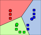
![2. [math]k[/math] clusters are created by associating every observation with the nearest mean. The partitions here represent the Voronoi diagram generated by the means.](/w/images/thumb/a/a5/K_Means_Example_Step_2.svg/139px-K_Means_Example_Step_2.svg.png)
2. [math]k[/math] clusters are created by associating every observation with the nearest mean. The partitions here represent the Voronoi diagram generated by the means.
-
![3. The centroid of each of the [math]k[/math] clusters becomes the new mean.](/w/images/thumb/0/0a/K_Means_Example_Step_33.svg/139px-K_Means_Example_Step_33.svg.png)
3. The centroid of each of the [math]k[/math] clusters becomes the new mean.
-
4. Steps 2 and 3 are repeated until convergence has been reached.
![1. [math]k[/math] initial "means" (in this case [math]k[/math]=3) are randomly generated within the data domain (shown in color).](/wiki/File:K_Means_Example_Step_1.svg)
![2. [math]k[/math] clusters are created by associating every observation with the nearest mean. The partitions here represent the Voronoi diagram generated by the means.](/wiki/File:K_Means_Example_Step_2.svg)
![3. The centroid of each of the [math]k[/math] clusters becomes the new mean.](/wiki/File:K_Means_Example_Step_33.svg)

Discussion
Three key features of [math]k[/math]-means that make it efficient are often regarded as its biggest drawbacks:
- Euclidean distance is used as a metric and variance is used as a measure of cluster scatter.
- The number of clusters [math]k[/math] is an input parameter: an inappropriate choice of [math]k[/math] may yield poor results.
- Convergence to a local minimum may produce counterintuitive ("wrong") results (see example in Fig.).

A key limitation of [math]k[/math]-means is its cluster model. The concept is based on spherical clusters that are separable so that the mean converges towards the cluster center. The clusters are expected to be of similar size, so that the assignment to the nearest cluster center is the correct assignment. When for example applying [math]k[/math]-means with a value of [math]k=3[/math] onto the well-known Iris flower data set, the result often fails to separate the three Iris species contained in the data set. With [math]k=2[/math], the two visible clusters (one containing two species) will be discovered, whereas with [math]k=3[/math] one of the two clusters will be split into two even parts. In fact, [math]k=2[/math] is more appropriate for this data set, despite the data set's containing 3 classes. As with any other clustering algorithm, the [math]k[/math]-means result makes assumptions that the data satisfy certain criteria. It works well on some data sets, and fails on others.

The result of [math]k[/math]-means can be seen as the Voronoi cells of the cluster means. Since data is split halfway between cluster means, this can lead to suboptimal splits as can be seen in the "mouse" example. The Gaussian models used by the expectation-maximization algorithm (arguably a generalization of [math]k[/math]-means) are more flexible by having both variances and covariances. The EM result is thus able to accommodate clusters of variable size much better than [math]k[/math]-means as well as correlated clusters (not in this example). In counterpart, EM requires the optimization of a larger number of free parameters and poses some methodological issues due to vanishing clusters or badly-conditioned covariance matrices.

References
- "The (black) art of runtime evaluation: Are we comparing algorithms or implementations?" (2016). Knowledge and Information Systems 52 (2): 341–378. doi:. ISSN 0219-1377.
- MacQueen, J. B. (1967). Some Methods for classification and Analysis of Multivariate Observations. Proceedings of 5th Berkeley Symposium on Mathematical Statistics and Probability. 1. University of California Press. pp. 281–297. MR 0214227. Zbl 0214.46201. Retrieved 2009-04-07.
- Steinhaus, Hugo (1957). "Sur la division des corps matériels en parties" (in fr). Bull. Acad. Polon. Sci. 4 (12): 801–804.
- Lloyd, Stuart P. (1957). "Least square quantization in PCM". Bell Telephone Laboratories Paper. Published in journal much later: Lloyd, Stuart P. (1982). "Least squares quantization in PCM". IEEE Transactions on Information Theory 28 (2): 129–137. doi:.
- Forgy, Edward W. (1965). "Cluster analysis of multivariate data: efficiency versus interpretability of classifications". Biometrics 21 (3): 768–769.
- "Accelerating exact k -means algorithms with geometric reasoning" (in en) (1999). Proceedings of the Fifth ACM SIGKDD International Conference on Knowledge Discovery and Data Mining - KDD '99: 277–281. San Diego, California, United States: ACM Press. doi:.
- MacKay, David (2003). "Chapter 20. An Example Inference Task: Clustering" (PDF). Information Theory, Inference and Learning Algorithms. Cambridge University Press. pp. 284–292. ISBN 978-0-521-64298-9. MR 2012999.
- Since the square root is a monotone function, this also is the minimum Euclidean distance assignment.
- "Algorithm AS 136: A [math]k[/math]-Means Clustering Algorithm" (1979). Journal of the Royal Statistical Society, Series C 28 (1): 100–108.
- 10.0 10.1 Hamerly, Greg; Elkan, Charles (2002). "Alternatives to the [math]k[/math]-means algorithm that find better clusterings" (PDF). Proceedings of the eleventh international conference on Information and knowledge management (CIKM).
- "A comparative study of efficient initialization methods for the [math]k[/math]-means clustering algorithm" (2013). Expert Systems with Applications 40 (1): 200–210. doi:.
- Bradley, Paul S.; Fayyad, Usama M. (1998). "Refining Initial Points for [math]k[/math]-Means Clustering". Proceedings of the Fifteenth International Conference on Machine Learning.
- Mirkes, E. M. "K-means and [math]k[/math]-medoids applet". Retrieved 2 January 2016.
Wikipedia References
- Wikipedia contributors. "K-means clustering". Wikipedia. Wikipedia. Retrieved 17 August 2022.